11.2 Unit Tangent and Principal Unit Normal Vectors; Arc LengthPrinted Page 767
767
A vector function \(\mathbf{r}=\mathbf{r}(t)\) that is defined on a closed interval \(a\leq t\leq b\) traces out a curve as \(t\) varies over the interval. In this section, we analyze the curve geometrically by defining a tangent vector and a normal vector to the curve. We also express the arc length of a curve in terms of the unit tangent vector \(\mathbf{T}.\)
RECALL
The terms normal, perpendicular, and orthogonal all mean “meet at right angles.”
1 Interpret the Derivative of a Vector Function GeometricallyPrinted Page 767
Suppose a vector function \(\mathbf{r}=\mathbf{r}(t)\) is defined on an interval \([ a,b]\) and is differentiable on \(( a,b).\) Then \(\mathbf{r}=\mathbf{r}( t)\) traces out a curve \(C\) as \(t\) varies over the interval. For a number \(t_{0}\), \(a<t_{0}<b,\) there is a point \(P_{0}\) on \(C\) given by the vector \(\mathbf{r}=\mathbf{r}(t_{0}).\) If \(h\neq 0\), there is a point \(Q\) on \(C\) different from \(P_{0}\) given by the vector \(\mathbf{r}(t_{0}+h).\) The vector \(\dfrac{\mathbf{r}(t_{0}+h)-\mathbf{r}(t_{0})}{h}\) can be thought of as a secant vector in the direction from \(P_{0}\) to \(Q\), as shown in Figure 8. Notice that whether \(h<0\) or \(h>0,\) the direction of the secant vectors follows the orientation of \(C.\)
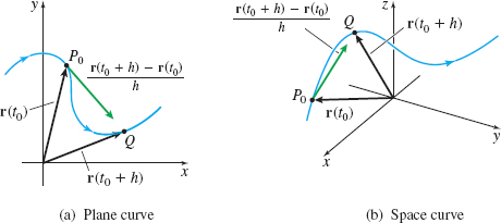
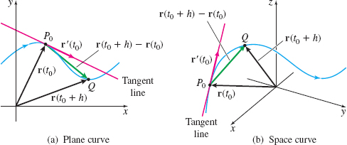
As \(h\rightarrow 0,\) the vector in the direction from \(P_{0}\) to \(Q\) moves along the curve \(C\) toward \(P_{0},\) getting closer and closer to the vector tangent to \(C\) at \(P_{0}\), as shown in Figure 9. The direction of the tangent vector follows the orientation of \(C.\) But as \(h\rightarrow 0,\) the vector \(\dfrac{\mathbf{r}( t_{0}+h) -\mathbf{r}( t_{0}) }{h}\) approaches the derivative \(\mathbf{r^{\prime} }( t_{0}) .\) This leads to the following definition.


768
NOTE
There is no tangent vector defined if \(\mathbf{r}^{\prime} (t_{0})=\mathbf{0}.\)
DEFINITION Tangent Vector to a Curve \(C\)
Suppose \(\mathbf{r}=\mathbf{r}(t)\) is a vector function defined on the interval \([ a,b] \) and differentiable on the interval \(( a,b) .\) Let \(P_{0}\) be the point on the curve \(C\) traced out by \(\mathbf{r}=\mathbf{r}(t)\) corresponding to \(t=t_{0},\) \(a<t_{0}<b.\) If \(\mathbf{r}^{\prime} (t_{0})\neq \mathbf{0}\), then the vector \(\mathbf{r^{\prime} }( t_{0}) \) is a tangent vector to the curve at \(t_{0}.\) The line containing \(P_{0}\) in the direction of \(\mathbf{r}^{\prime} (t_{0})\) is the tangent line to the curve traced out by \(\mathbf{r}=\mathbf{r}(t)\) at \(t_{0}.\)
RECALL
The angle between two nonzero vectors \(\mathbf{v}\) and \(\mathbf{w}\) is determined by \(\cos \theta =\dfrac{\mathbf{v}\,{\cdot}\,\mathbf{w}} {\left\Vert \mathbf{v}\right\Vert \left\Vert \mathbf{w}\right\Vert }\), where \(0\leq \theta \leq \pi.\)
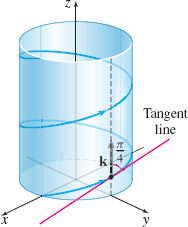
EXAMPLE 1Finding the Angle Between a Tangent Vector to a Helix and the Direction \(\mathbf{k}\)
Show that the acute angle between the tangent vector to the helix \[ \mathbf{r}(t)=\cos t\mathbf{i}+\sin t\mathbf{j}+t\mathbf{k}\quad 0\,{\leq}\,t\,{\leq}\,2\pi \]
and the direction \(\mathbf{k}\) is \(\dfrac{\pi }{4}\) radian.
Solution A tangent vector at any point on the helix is given by \begin{equation*} \mathbf{r}^{\prime} (t)=-\sin t\mathbf{i}+\cos t\mathbf{j}+\mathbf{k} \end{equation*}
Then \(\left\Vert \mathbf{r}^{\prime} (t)\right\Vert\;= \sqrt{(-\sin t)^2 + \cos^2 t +1} = \sqrt{1+1} = \sqrt{2}.\)
The cosine of the acute angle \(\theta \) between \(\mathbf{r}^{\prime} (t)\) and \(\mathbf{k}\) is \begin{eqnarray*} &&\cos \theta =\frac{\mathbf{r}^{\prime} (t)\,{\cdot}\, \mathbf{k}}{\left\Vert \mathbf{r} ^{\prime} (t)\right\Vert \left\Vert \mathbf{k}\right\Vert }=\frac{1}{\sqrt{2}}=\frac{\sqrt{2}}{2}\qquad \color{#0066A7}{\hbox{$\mathbf{r}^{\prime} (t)\,{\cdot}\, \mathbf{k} = 1$}}\\ \end{eqnarray*}
So, \(\theta =\dfrac{\pi }{4}\) radian. See Figure 10.
NOW WORK
2 Find the Unit Tangent Vector and the Principal Unit Normal Vector of a Smooth CurvePrinted Page 768
We now state the definition of a smooth curve in terms of vector functions. You may wish to compare this definition with the one given in Section 9.2, p. 647.
DEFINITION Smooth Curve
Let \(C\) denote a curve traced out by a vector function \(\mathbf{r}=\mathbf{r}(t)\) that is continuous for \(a\leq t\leq b.\) If the derivative \(\mathbf{r}^{\prime} (t)\) exists and is continuous on the interval \(( a,b) \) and if \(\mathbf{r}^{\prime} (t)\) is never \(\mathbf{0}\) on \(( a,b), \) then \(C\) is called a smooth curve.
Since \(\mathbf{r}^{\prime} ( t) \) is never \(\mathbf{0}\) for a smooth curve, such curves will have tangent vectors at every point.
The unit tangent vector and the unit normal vector are important for analyzing the geometry of a curve (Section 11.3) and for describing motion along a curve (Section 11.4).
For a smooth curve \(C\) traced out by the vector function \(\mathbf{r}=\mathbf{r}(t)\), \(a\leq t\leq b\), the unit tangent vector \(\mathbf{T}(t)\) to \(C\) at \(t\) is \begin{equation*} \bbox[5px, border:1px solid black, #F9F7ED] {\mathbf{T}(t)=\dfrac{\mathbf{r}^{\prime} (t)}{\left\Vert \mathbf{r}^{\prime} (t)\right\Vert}} \end{equation*}
769

EXAMPLE 2Finding a Unit Tangent Vector to a Curve
Show that the unit tangent vector \(\mathbf{T}(t)\) to the circle of radius \(R\) \begin{equation*} \mathbf{r}(t)=R\cos t\mathbf{i}+R\;\sin t\mathbf{j}\quad 0\leq t\leq 2\pi \end{equation*}
is everywhere orthogonal to \(\mathbf{r}(t).\) Graph \(\mathbf{r}=\mathbf{r}( t)\) and \(\mathbf{T}=\mathbf{T}( t).\)
Solution We begin by finding \(\mathbf{r}^{\prime} (t)\) and \(\left\Vert \mathbf{r}^{\prime} (t)\right\Vert\): \begin{eqnarray*} \mathbf{r}^{\prime} (t)& =&\dfrac{d}{dt}( R\cos t) \mathbf{i}+ \dfrac{d}{dt}( R\;\sin t) \mathbf{j}=-R\;\sin t\mathbf{i}+R\cos t\mathbf{j} \\[6pt] \left\Vert \mathbf{r}^{\prime} (t)\right\Vert & =&\sqrt{(-R\;\sin t)^{2}+(R\cos t)^{2}}=R \end{eqnarray*}
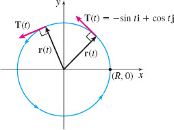
Then the unit tangent vector is \begin{equation*} \mathbf{T}(t)=\frac{\mathbf{r}^{\prime} (t)}{\left\Vert \mathbf{r}^{\prime} (t)\right\Vert }=\dfrac{-R\;\sin t\mathbf{i}+R\;\cos t\mathbf{j}}{R}=-\!\sin t\mathbf{i}+\cos t\mathbf{j} \end{equation*}
To determine whether \(\mathbf{r}( t)\) is orthogonal to \(\mathbf{T}( t), \) we find their dot product. \begin{equation*} \mathbf{T}(t)\,{\cdot}\, \mathbf{r}(t)=( -\!\sin t\mathbf{i}+\cos t\mathbf{j}) \,{\cdot}\, ( R\;\cos t\mathbf{i}+R\;\sin t\mathbf{j}) =-R\;\sin t\cos t+R\;\sin t\cos t=0 \end{equation*}
for all \(t.\) That is, \(\mathbf{T}(t)\) is everywhere orthogonal to \(\mathbf{r}(t)\), as shown in Figure 11.
The following discussion leads to the definition of the principal unit normal vector.
Suppose a smooth curve \(C\) is traced out by a twice differentiable vector function \(\mathbf{r}=\mathbf{r}(t).\) Then the unit tangent vector \(\mathbf{T}(t)\) is differentiable. Also, since \(\mathbf{T}(t)\) is a unit vector, \[ \mathbf{T}(t)\,{\cdot}\, \mathbf{T}(t)=1\quad \hbox{for all}\,t \]
If we differentiate this expression, we find \[ \begin{array}{rcl@{\qquad}l} \dfrac{d}{dt}[\mathbf{T}(t)\,{\cdot}\, \mathbf{T}(t)]& =&\dfrac{d}{dt}( 1) & \color{#0066A7}{\hbox{Differentiate both sides.}} \\[12pt] \mathbf{T}^{\prime} (t)\,{\cdot}\, \mathbf{T}(t)+\mathbf{T}(t)\,{\cdot}\, \mathbf{T}^{\prime} (t) &=& 0 & \color{#0066A7}{\hbox{Use the dot product rule.}} \\[6pt] \mathbf{T}(t)\,{\cdot}\, \mathbf{T}^{\prime} (t)& =&0 & \color{#0066A7}{\hbox{Simplify.}} \end{array} \]
We conclude that \(\mathbf{T}^{\prime} (t)\) is a vector that is orthogonal to \(\mathbf{T}(t)\) at every point on the \(C\). In particular, the vector \(\dfrac{\mathbf{T}^{\prime} (t)}{\left\Vert \mathbf{T}^{\prime} (t)\right\Vert }\) is a unit vector that is orthogonal to \(\mathbf{T}(t)\) at every point on the curve \(C.\)
DEFINITION Principal Unit Normal Vector
For a smooth curve \(C\) traced out by a vector function \(\mathbf{r}=\mathbf{r}(t),\) \(a\leq t\leq b,\) that is twice differentiable for \(a<t<b,\) the principal unit normal vector \(\mathbf{N}(t)\) to \(C\) at \(t\) is \begin{equation*} \bbox[5px, border:1px solid black, #F9F7ED] {\mathbf{N}(t)=\dfrac{\mathbf{T}^{\prime} (t)}{\left\Vert \mathbf{T}^{\prime} (t)\right\Vert }} \end{equation*}
Notice that the unit normal vector \(\mathbf{N}\) is not defined if \(\mathbf{T^{\prime} =0.}\) So, for example, lines do not have well-defined unit normals.
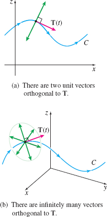
If \(C\) is a plane curve, there are two unit vectors that are orthogonal to the unit tangent vector \(\mathbf{T}\), as shown in Figure 12(a). If \(C\) is a curve in space, there are infinitely many unit vectors that are orthogonal to the unit tangent vector \(\mathbf{T}\), as shown in Figure 12(b). The definition of the principal unit normal vector identifies exactly one of the orthogonal vectors and gives it a name.
770
EXAMPLE 3Finding the Principal Unit Normal Vector
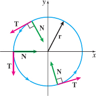
Find the principal unit normal vector \(\mathbf{N}(t)\) to the circle \(\mathbf{r}( t) =R\;\cos t\mathbf{i}+R\;\sin t\mathbf{j}\), \(0\leq t\leq 2\pi .\) (Refer to Example 2.) Graph \(\mathbf{r}=\mathbf{r}( t), \) and show a unit tangent vector and a unit normal vector.
Solution From Example 2, the unit tangent vector \(\mathbf{T}(t)\) is \begin{equation*} \mathbf{T}(t)=-\!\sin t\mathbf{i}+\cos t\mathbf{j} \end{equation*}
Since \(\mathbf{T}^{\prime} ( t) =-\cos t\mathbf{i}-\sin t\mathbf{j},\) the principal unit normal vector \(\mathbf{N}(t)\) is \begin{equation*} \mathbf{N}(t)=\frac{\mathbf{T}^{\prime} (t)}{\left\Vert \mathbf{T}^{\prime} (t)\right\Vert }=\frac{-\!\cos t\mathbf{i}-\sin t\mathbf{j}}{\sqrt{(-\!\cos t)^{2}+(-\!\sin t)^{2}}}=-\cos t\mathbf{i}-\sin t\mathbf{j} \end{equation*}
Since \(\mathbf{r}( t) = R ( \cos t\mathbf{i}+\sin t\mathbf{j}), \) the vector \(\mathbf{N}( t)\) is parallel to \(-\mathbf{r}(t)\). That is, \(\mathbf{N}(t)\) is a unit vector opposite in direction to the vector \(\mathbf{r}(t)\), so \(\mathbf{N}\) is directed toward the center of the circle, as shown in Figure 13.
NOW WORK
EXAMPLE 4Finding the Principal Unit Normal Vector of a Helix
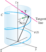
Show that the principal unit normal vector \(\mathbf{N}(t)\) of the helix \begin{equation*} \mathbf{r}(t)=\cos t\mathbf{i}+\sin t\mathbf{j}+t\mathbf{k} \end{equation*}
is orthogonal to the \(z\)-axis.
Solution We begin by finding \(\mathbf{r^{\prime} }( t) \) and \(\left\Vert \mathbf{r}^{\prime} ( t)\right \Vert.\) \[ \begin{equation*} \mathbf{r}^{\prime} (t)=-\!\sin t\mathbf{i}+\cos t\mathbf{j}+\mathbf{k}\qquad \left\Vert \mathbf{r}^{\prime }(t)\right\Vert =\sqrt{ (-\!\sin t)^{2}+(\cos t)^{2}+1}=\sqrt{2} \end{equation*} \]
Then the unit tangent vector is \(\mathbf{T}(t)=\dfrac{\mathbf{r}^{\prime }(t)}{||\mathbf{r}^{\prime }(t)||}=\dfrac{-\!\sin t\mathbf{i}+\cos t\mathbf{j}+\mathbf{k}}{\sqrt{2}}.\)
Since \[ \begin{equation*} \mathbf{T}^{\prime} (t)=\dfrac{-\!\cos t\mathbf{i}-\sin t\mathbf{j}}{\sqrt{2} }\qquad \hbox{and}\qquad \left\Vert \mathbf{T}^{\prime }(t)\right\Vert =\sqrt{ \left( -\dfrac{\cos t}{\sqrt{2}}\right) ^{2}+\left( -\dfrac{\sin t}{\sqrt{2}} \right) ^{2}}=\dfrac{1}{\sqrt{2}} \end{equation*} \]
we have \begin{equation*} \mathbf{N}(t)=\dfrac{\mathbf{T}^{\prime} (t)}{\left\Vert \mathbf{T}^{\prime} (t)\right\Vert }=-\!\cos t\mathbf{i}-\sin t\mathbf{j} \end{equation*}
Since the direction of the \(z\)-axis is \(\mathbf{k}\), it follows that \(\mathbf{N}(t)\,{\cdot}\, \mathbf{k}=0\) for all \(t.\) So, \(\mathbf{N}(t)\) is always orthogonal to the \(z\)-axis, as shown in Figure 14.
NOW WORK
3 Find the Arc Length of a Curve Traced Out by a Vector FunctionPrinted Page 770
A formula for the arc length of a smooth plane curve was derived in Chapter 9. The formula for the arc length of a smooth curve traced out by a vector function is given next.
THEOREM Arc Length of a Vector Function
If a smooth curve \(C\) is traced out by the vector function \(\mathbf{r}=\mathbf{r}(t),\) \(a\leq t\leq b\), the arc length \(s\) along \(C\) from \(t=a\) to \(t=b\) is \begin{equation*} \bbox[5px, border:1px solid black, #F9F7ED] {s=\int_{a}^{b}\left\Vert \mathbf{r}^{\prime} (t)\right\Vert dt} \end{equation*}
771
For a smooth plane curve \(C\), traced out by \[ \mathbf{r}(t)=x(t)\mathbf{i}+y(t)\mathbf{j}\qquad a\leq t\leq b \]
we have \[ \mathbf{r}^{\prime} (t)=\dfrac{dx}{dt}\mathbf{i}\,{+}\,\dfrac{dy}{dt}\mathbf{j}\qquad \hbox{and}\qquad \left\Vert \mathbf{r^{\prime} }( t)\right\Vert =\;\sqrt{ \left( \dfrac{dx}{dt}\right) ^{2}+\left( \dfrac{dy}{dt}\right) ^{2}} \]
NEED TO REVIEW?
The arc length of a smooth curve is discussed in Section 9.2, pp. 651-653.
The arc length of \(C\) from \(a\) to \(b\) is given by \begin{equation*} s=\int_{a}^{b}\sqrt{\left( \dfrac{dx}{dt}\right) ^{2}+\left( \dfrac{dy}{dt} \right) ^{2}}\,\,dt=\int_{a}^{b}\Vert \mathbf{r}^{\prime} ( t) \Vert dt \end{equation*}
For a smooth space curve \(C\), traced out by \[ \mathbf{r}(t)=x(t)\mathbf{i}+y(t)\mathbf{j}+z(t)\mathbf{k}\qquad a\leq t\leq b \]
we have \[ \mathbf{r^{\prime} }(t)=\dfrac{dx}{dt}\mathbf{i}+\dfrac{dy}{dt}\mathbf{j}+ \dfrac{dz}{dt}\mathbf{k}\qquad \hbox{and}\qquad \left\Vert \mathbf{r^{\prime} }( t) \right\Vert =\sqrt{\left( \dfrac{dx}{dt}\right) ^{2}+\left( \dfrac{ dy}{dt}\right) ^{2}+\left( \dfrac{dz}{dt}\right) ^{2}} \]
The arc length of \(C\) from \(a\) to \(b\) is given by \begin{equation*} s=\int_{a}^{b}\sqrt{\left( \dfrac{dx}{dt}\right) ^{2}+\left( \dfrac{dy}{dt} \right) ^{2}+\left( \dfrac{dz}{dt}\right) ^{2}}\,\,dt=\int_{a}^{b}\left\Vert \mathbf{r}^{\prime} ( t) \right\Vert dt \end{equation*}
EXAMPLE 5Finding the Arc Length of a Circle and a Helix
Find the arc length of:
(a) The circle \(\mathbf{r}(t)=R\;\cos t\mathbf{i}+R\;\sin t\mathbf{j}\) from \(t=0\) to \(t=2\pi \)
(b) The circular helix \(\mathbf{r}(t)=R\;\cos t\mathbf{i}+R\;\sin t\mathbf{j}+t\mathbf{k}\) from \(t=0\) to \(t=2\pi \)
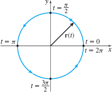
Solution (a) We begin by finding \(\mathbf{r^{\prime} }( t)\) and \(\left\Vert \mathbf{r^{\prime} }( t) \right\Vert \): \[ \mathbf{r}^{\prime} (t)=-R\;\sin t\mathbf{i}+R\;\cos t\mathbf{j}\qquad \left\Vert \mathbf{r}^{\prime} (t)\right\Vert =\sqrt{(-R\;\sin t)^{2}+(R\;\cos t)^{2}}=R \]
Now we use the formula for arc length. \begin{equation*} s=\int_{a}^{b}\left\Vert \mathbf{r}^{\prime} (t)\right\Vert dt=\int_{0}^{2\pi }Rdt=\big[ R\hbox{ }t\big] _{0}^{2\pi }=2\pi R \end{equation*}
which is the familiar formula for the circumference of a circle. See Figure 15.
(b) We begin by finding \(\mathbf{r^{\prime} }( t)\) and \(\left\Vert \mathbf{r^{\prime} }( t) \right\Vert.\) \begin{eqnarray*} \mathbf{r}^{\prime} (t) &=&-R\;\sin t\mathbf{i}\,{+}\,R\;\cos t\mathbf{j}+\mathbf{k},\\[6pt] \left\Vert \mathbf{r}^{\prime} (t)\right\Vert &=& \sqrt{\!(-R\;\sin t)^{2}\,{+}\,(R\;\cos t)^{2}\,{+}\,1^{2}}\,{=}\,\sqrt{R^{2}\,{+}\,1} \end{eqnarray*}
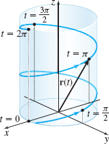
Then \begin{equation*} ~s=\int_{a}^{b}\left\Vert \mathbf{r}^{\prime} ( t) \right\Vert dt=\int_{0}^{2\pi }\sqrt{R^{2}+1}~dt=\left[ \sqrt{R^{2}+1}\,t\right] _{0}^{2\pi }=2\pi \sqrt{R^{2}+1} \end{equation*}
See Figure 16.
NOW WORK
For most vector functions, finding arc length requires technology.
772
EXAMPLE 6Using Technology to Find the Arc Length of an Ellipse
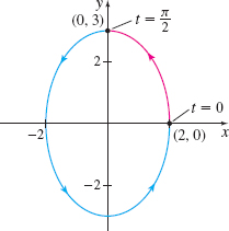
![]() Use technology to find the arc length \(s\) of the ellipse shown in Figure 17 traced out by the vector function \(\mathbf{r}( t) =2\cos t\mathbf{i}+3\sin t\mathbf{j}\) from \(t=0\) to \(t=\dfrac{\pi }{2}.\)
Use technology to find the arc length \(s\) of the ellipse shown in Figure 17 traced out by the vector function \(\mathbf{r}( t) =2\cos t\mathbf{i}+3\sin t\mathbf{j}\) from \(t=0\) to \(t=\dfrac{\pi }{2}.\)
Solution We begin by finding \(\mathbf{r^{\prime} }( t) \) and \(\left\Vert \mathbf{r^{\prime} }( t) \right\Vert .\) \[ \mathbf{r}^{\prime} (t)=-2\sin t\mathbf{i}+3\cos t\mathbf{j}\qquad \left\Vert \mathbf{r}^{\prime} (t)\right\Vert =\sqrt{4\sin ^{2}t+9\cos ^{2}t} \]
Now we use the formula for arc length. \begin{equation*} s=\int_{a}^{b}\left\Vert \mathbf{r}^{\prime} (t)\right\Vert dt=\int_{0}^{\pi /2}\sqrt{4\sin ^{2}t+9\cos ^{2}t}\,dt \end{equation*}
This is an integral that has no antiderivative in terms of elementary functions. To obtain a numerical approximation to the arc length, we use a CAS or a graphing utility.
When entering the integral in WolframAlpha, we find \begin{equation*} \int_{0}^{\pi /2}\sqrt{4\sin ^{2}t+9\cos ^{2}t}\,dt\approx 3.96636 \end{equation*}
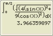
If we use a TI-84 to find the value of this integral, we obtain the same result. The screen shot is given in Figure 18.