Section 12.1 Exercises
CLARIFYING THE CONCEPTS
Question 12.1
1. Does the overall sample mean always equal the mean of the sample means? Explain. (p. 670)
12.1.1
No. If the sample sizes are not all the same, then we need to calculate the overall sample mean by calculating the weighted mean of the sample means where the weights are the sample sizes.
Question 12.2
2. What does MSTR measure? What does MSE measure? (p. 671)
Question 12.4
4. What are the required conditions for performing an analysis of variance? (p. 668)
Question 12.5
5. A comparison dotplot of the SAT scores of three sororities shows no overlap at all between the groups. Does this represent evidence for or against the null hypothesis that all population means are equal? (p. 667)
12.1.5
Against.
Question 12.6
6. True or false: If we reject the null hypothesis in an analysis of variance, then there is evidence that all the population mean sizes are different. If the statement is false, explain why it is false. (p. 673)
PRACTICING THE TECHNIQUES
 CHECK IT OUT!
| To do | Check out | Topic |
|---|---|---|
| Exercises 7–10 | Example 1 | Verifying the requirements for ANOVA |
| Exercises 11–14 | Example 2 | Calculating the overall sample mean ˉˉx |
| Exercises 15–22 | Example 3 | Constructing the ANOVA table |
| Exercises 23–28 | Example 4 | One-way ANOVA: p-value method |
| Exercises 29–30 | Example 6 | One-way ANOVA: critical-value method |
For Exercises 7–10, assume that the samples were drawn independently and confirm that the other requirements for ANOVA are met by doing the following:
- Use technology to construct a probability plot for each group. Check for normality.
- Check for equal variances.
Question 12.7
7.
| A | B | C |
|---|---|---|
| 5 | 10 | 15 |
| 10 | 15 | 20 |
| 15 | 20 | 25 |
12.1.7
(a)
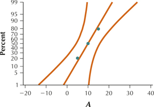
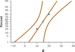
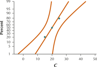
All three graphs show acceptable normality.
(b)
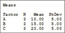
All three standard deviations are equal to 5, so all of them are less than 2(5.00)=10.00. Therefore, the equal variance requirement is satisfied.
Question 12.8
8.
| A | B | C |
|---|---|---|
| 10 | 12 | 14 |
| 20 | 18 | 20 |
| 30 | 30 | 26 |
Question 12.9
9.
| A | B | C | D |
|---|---|---|---|
| 30 | 35 | 45 | 5 |
| 0 | 75 | 20 | 30 |
| 25 | 55 | 10 | 0 |
| 0 | 45 | 25 | 35 |
12.1.9
(a)
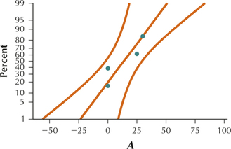
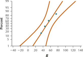
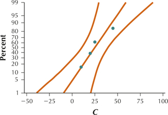
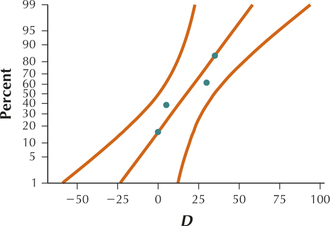
All four graphs show acceptable normality.
(b)
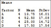
The smallest standard deviation is 14.72 which is the standard deviation for group C. Twice 14.72 is 29.44. All other standard deviations are less than 29.44 so the equal variance requirement is satisfied.
Question 12.10
10.
| A | B | C | D |
|---|---|---|---|
| 5 | 8 | 3 | 6 |
| 2 | 7 | 7 | 4 |
| 4 | 10 | 5 | 5 |
| 1 | 6 | 4 | 3 |
| 3 | 9 | 6 | 7 |
For Exercises 11–14, calculate the overall sample mean ˉˉx for the indicated data.
Question 12.11
11. Data in Exercise 7
12.1.11
ˉˉx=15
Question 12.12
12. Data in Exercise 8
Question 12.13
13. Data in Exercise 9
12.1.13
ˉˉx=27.1875
Question 12.14
14. Data in Exercise 10
For Exercises 15–22, do the following for the indicated data.
- Calculate the following:
- SSTR=Σni(ˉx−ˉˉx)2
- SSE=Σ(ni−1)s2i
- SST=SSTR+SSE
- df1=k−1
- df2=nt−k
- MSTR=SSTR/df1
- MSE=SSE/df2
- Construct the ANOVA table using the statistics computed in (a).
Question 12.15
15. Data in Exercise 7
12.1.15
(a) (i) SSTR = 150 (ii) SSE = 150 (iii) SST = 300 (iv) df1=2 (v) df2=6 (vi) MSTR = 75 (vii) MSE = 25
(b)

Question 12.16
16. Data in Exercise 8
Question 12.17
17. Data in Exercise 9
12.1.17
(a) (i) SSTR = 3680 (ii) SSE = 3219 (iii) SST = 6898 (iv) df1=3 (v) df2=12 (vi) MSTR = 1226.6 (vii) MSE = 268.2
(b)

Question 12.18
18. Data in Exercise 10
Question 12.19
19.
| Sample A | Sample B | Sample C |
|---|---|---|
| ˉxA=10 | ˉxB=12 | ˉxC=8 |
| sA=1 | sB=1 | sC=1 |
| nA=5 | nB=5 | nC=5 |
12.1.19
(a) (i) SSTR = 40 (ii) SSE = 12 (iii) SST = 52 (iv) df1=2 (v) df2=12 (vi) MSTR = 20 (vii) MSE = 1
(b)
| Source of variation |
Sum of squares |
Degrees of freedom |
Mean square |
F |
|---|---|---|---|---|
| Treatments | 40 | 2 | 20 | 20 |
| Error | 12 | 12 | 1 | |
| Total | 52 |
Question 12.20
20.
| Sample A | Sample B | Sample C | Sample D |
|---|---|---|---|
| ˉxA=10 | ˉxB=12 | ˉxC=8 | ˉxD=14 |
| sA=1 | sB=1 | sC=1 | sD=1 |
| nA=5 | nB=5 | nC=5 | nD=5 |
Question 12.21
21.
| Sample A | Sample B | Sample C | Sample D |
|---|---|---|---|
| ˉxA=50 | ˉxB=75 | ˉxC=100 | ˉxD=125 |
| sA=5 | sB=4 | sC=6 | sD=5 |
| nA=100 | nB=150 | nC=200 | nD=150 |
12.1.21
(a) (i) SSTR = 395,833.3333 (ii) SSE = 15,748 (iii) SST = 411,581.3333 (iv) df1=3 (v) df2=596 (vi) MSTR = 131,944.4444 (vii) MSE = 26.4228
(b)
| Source of variation |
Sum of squares |
Degrees of freedom |
Mean square |
F |
|---|---|---|---|---|
| Treatments | 395,833.3333 | 3 | 131,944.4444 | 4993.5794 |
| Error | 15,748 | 594 | 26.4228 | |
| Total | 411,581.3333 |
Question 12.22
22.
| Sample A | Sample B | Sample C | Sample D |
|---|---|---|---|
| ˉxA=0 | ˉxB=10 | ˉxC=20 | ˉxD=10 |
| sA=1.5 | sB=2.25 | sC=1.75 | sD=2.0 |
| nA=50 | nB=100 | nC=50 | nD=100 |
For Exercises 23–30, assume that the ANOVA assumptions are verified.
For the ANOVA table indicated in Exercises 23–28, test whether the population means differ, using the p-value method and α=0.05.
Question 12.23
23. ANOVA table from Exercise 15
12.1.23
H0:μA=μB=μC versus Ha: Not all the population means are equal.
Reject H0 if the p-value≤α=0.05.
Fdata=3.00.
p-value= 0.125.
The p-value= 0.125 is not ≤α=0.05. Therefore we do not reject H0. There is not enough evidence to conclude at level of significance α=0.05 that the population means are not all equal.
Question 12.24
24. ANOVA table from Exercise 16
Question 12.25
25. ANOVA table from Exercise 17
12.1.25
H0:μA=μB=μC=μD versus Ha: Not all the population means are equal.
Reject H0 if the p-value≤α=0.05.
Fdata=4.57.
p-value= 0.023.
The p-value= 0.023 is ≤α=0.05. Therefore we reject H0. There is evidence at level of significance α=0.05 that the population means are not all equal.
Question 12.26
26. ANOVA table from Exercise 18
Question 12.27
27. ANOVA table from Exercise 19
12.1.27
H0:μA=μB=μC
Ha: Not all the population means are equal.
Reject H0 if the p-value≤α=0.05.
Fdata=20.
p-value= 0.0002.
The p-value= 0.0002 is ≤α=0.05. Therefore we reject H0. There is evidence at level of significance α=0.05 that the population means are not all equal.
Question 12.28
28. ANOVA table from Exercise 20
For the data indicated in Exercises 29–30, test whether the population means differ, using the critical-value method and α=0.01.
Question 12.29
29. ANOVA table from Exercise 21
12.1.29
H0:μA=μB=μC=μD;
Ha: Not all the population means are equal.
Fcrit=3.815 Reject H0 if Fdata≥.0815;
Fdata=4793.5794;
Fdata=4793.5794 is ≥3.815. Therefore we reject H0. There is evidence at level of significance α=0.01 that the population means are not all equal.
Question 12.30
30. ANOVA table from Exercise 22
APPLYING THE CONCEPTS
For Exercises 31–34, assume that the data are independently drawn random samples from normal populations.
- Verify the equal-variance assumption.
- Calculate the following measures:
- df1 and df2
- ˉˉx
- SSTR
- SSE
- SST
- MSTR
- MSE
- Fdata
- Construct the ANOVA table.
- Perform the appropriate one-way ANOVA using level of significance α=0.05.
Question 12.31
cafeanova
31. Student-Run Café Business. In Example 8 in Chapter 2, we looked at data from a student-run café business. The table contains the number of food items sold per day.
| Wraps | Muffins | Chips |
|---|---|---|
| 12 | 6 | 7 |
| 13 | 3 | 16 |
| 19 | 10 | 8 |
| 5 | 1 | 4 |
| 22 | 8 | 10 |
12.1.31
(a)

The smallest standard deviation is 3.65, which is the standard deviation for muffins. Twice 3.65 is 7.30. All other standard deviations are less than 7.30, so the equal variance requirement is satisfied.
(b) (i) df1=2, df2=12 (ii) ˉˉx=9.6 (iii) SSTR = 187.6 (iv) SSE = 308 (v) SST = 495.6 (vi) MSTR = 93.80 (vii) MSE = 25.67 (viii) Fdata=3.65
(c)

(d) H0:μWraps=μMuffins=μChips;
Ha: Not all the population means are equal.
Reject H0 if the p-value≤α=0.05.
Fdata=3.65.
p-value= 0.058.
The p-value= 0.058 is not ≤α=0.05. Therefore we do not reject H0. There is not enough evidence to conclude at level of significance α=0.05 that the population means of the number of different types of food items are not all equal.
Question 12.32
prosdartsanova
32. The professionals versus the Darts. In the Chapter 3 Case Study, we examined stock market returns for professional financial analysts, compared to random darts and the Dow Jones Industrial Average (DJIA). The table contains daily stock market returns.
| Pros | Darts | DJIA |
|---|---|---|
| 10.6 | 20.6 | 4.4 |
| 27.8 | 18.5 | 11.2 |
| 29.1 | 1.8 | 3.7 |
| 2.2 | 11.7 | 17.6 |
| 14.1 | 1.8 | 0.2 |
Question 12.33
weightages
33. Weight and Age. The Chapter 4 Case Study looked at body measurements for physically fit males and females. Is there a difference in weight among different age groups? The table contains the weights of five randomly chosen females from each of three age groups: younger (18-22), middle (23-30), and older (31+).
| Younger | Middle | Older |
|---|---|---|
| 119 | 142.9 | 121.3 |
| 124.8 | 104.3 | 107.4 |
| 130.7 | 115.1 | 169.3 |
| 130.1 | 98.8 | 122.8 |
| 155.4 | 110.2 | 155.4 |
12.1.33
(a)

The smallest standard deviation is 13.91, which is the standard deviation for the younger. Twice 13.91 is 27.82. All other standard deviations are less than 27.82, so the equal variance requirement is satisfied.
(b) (i) df1=2, df2=12 (ii) ˉˉx=127.17 (iii) SSTR = 1276 (iv) SSE = 4640 (v) SST = 5916 (vi) MSTR = 637.8 (vii) MSE = 386.7 (viii) Fdata=1.65
(c)

(d) H0:μYounger=μMiddle=μOlder;
Ha: Not all the population means are equal.
Reject H0 if the p-value≤α=0.05.
Fdata=1.65.
p-value= 0.233.
The p-value= 0.233 is not ≤α=0.05. Therefore we do not reject H0. There is not enough evidence to conclude at level of significance α=0.05 that the population mean weights of the different age groups are not all equal.
Question 12.34
fullmoon
34. The Full Moon and Emergency Room Visits. Is there a difference in emergency room visits before, during, and after a full moon? A study looked at the admission rate (number of patients per day) to the emergency room of a Virginia mental health clinic over a series of 12 full moons.2 The data are provided in the table. Is there evidence of a difference in emergency room visits before, during, and after the full moon?
| Before | During | After | |||
|---|---|---|---|---|---|
| 6.4 | 11.5 | 5 | 13 | 5.8 | 13.5 |
| 7.1 | 13.8 | 13 | 16 | 9.2 | 13.1 |
| 6.5 | 15.4 | 14 | 25 | 7.9 | 15.8 |
| 8.6 | 15.7 | 12 | 14 | 7.7 | 13.3 |
| 8.1 | 11.7 | 6 | 14 | 11.0 | 12.8 |
| 10.4 | 15.8 | 9 | 20 | 12.9 | 14.5 |
Question 12.35
35. Missing Values. Part of an ANOVA table for an analysis of variance involving 7 groups for a study follows; each sample contained 10 data values.
| Source of variation |
Sum of square |
Degrees of freedom |
Mean squares |
F |
|---|---|---|---|---|
| Treatment | 120 | — | — | — |
| Error | 315 | — | — | |
| Total | — |
- Find all six missing values in the table and fill in the blanks.
- Perform the appropriate hypothesis test using α=0.05.
12.1.35
(a) Missing values are in red.
| Source of variation |
Sum of squares |
Degrees of freedom |
Mean square |
F |
|---|---|---|---|---|
| Treatments | 120 | 6 | 20 | 4 |
| Error | 315 | 63 | 5 | |
| Total | 435 |
(b) H0:μ1=μ2=μ3=μ4=μ5=μ6=μ7. Ha: Not all the population means are equal. Reject H0 if the p-value≤0.05. Fdata=4 p-value= 0.0018680725. Since the p-value≤0.05, we reject H0. There is evidence that not all the population means are equal.
Question 12.36
36. Missing Values. Part of an ANOVA table for an analysis of variance involving three groups follows; each sample contained six data values.
| Source of variation |
Sum of square |
Degrees of freedom |
Mean squares |
F |
|---|---|---|---|---|
| Treatment | — | — | — | — |
| Error | 90 | — | — | |
| Total | 150 |
- Find all six missing values in the table.
- Perform the appropriate hypothesis test using α=0.01.
Question 12.37
37. Missing Values. Part of an ANOVA table follows.
| Source of variation |
Sum of square |
Degrees of freedom |
Mean squares |
F |
|---|---|---|---|---|
| Treatment | — | 4 | 10 | 1.0 |
| Error | — | — | — | |
| Total | 440 |
- Find all four missing values in the table and fill in the blanks.
- Perform the appropriate hypothesis test using α=0.10.
12.1.37
(a) Missing values are in red.
| Source of variation |
Sum of squares |
Degrees of freedom |
Mean square |
F-test statistic |
|---|---|---|---|---|
| Treatments | SSTR = 40 | df1=4 | MSTR = 10 | Fdata=1.0 |
| Error | SSE = 400 | df2=40 | MSE = 10 | |
| Total | SST = 440 |
(b) H0:μ1=μ2=μ3=μ4=μ5. Ha: Not all the population means are equal. Fcrit=2.09. Reject H0 if Fdata≥2.09. Fdata=1.0. Since Fdata is not ≥2.09 we do not reject H0. There is insufficient evidence that not all the population means are equal.
Question 12.38
38. Missing Values. Part of an ANOVA table follows.
| Source of variation |
Sum of square |
Degrees of freedom |
Mean squares |
F |
|---|---|---|---|---|
| Treatment | — | 2 | — | 2.0 |
| Error | 480 | — | 24 | |
| Total | — |
- Find all four missing values in the table and fill in the blanks.
- Perform the appropriate hypothesis test using α=0.05.
Question 12.39
39. ANOVA Can Be Applied to Two populations. Researchers are interested in whether the mean heart rates of women and men differ. The following table provides summary statistics of random samples of pulse rates drawn from groups of women and men.
- Test, using α=0.05, whether the population mean pulse rates differ.
- Which method of inference from an earlier chapter could we also use to solve this problem?
| Females | Males | |
|---|---|---|
| n | 65 | 65 |
| ˉx | 98.384 | 98.104 |
| s | 0.743 | 0.699 |
12.1.39
(a) H0:μFemales=μMales. Ha: The two population means are not equal. μFemales = the population mean heart rate for females; μMales = the population mean heart rate for males. Reject H0 if the p-value≤0.05. Fdata=4.89693413, p-value= 0.0287. Since the p-value is ≤0.05, we reject H0. There is evidence that the population mean heart rates are not equal.
(b) Inference for Two Independent Means, Section 10.2.
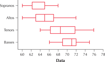
Do Taller people Have lower Voices? Use this information for Exercises 40 and 41. The heights of the members of the New York Choral Society were recorded.3 Choral singers are roughly divided into four groups, from highest-pitched voices to lowest: sopranos and altos (usually female), and tenors and basses (usually male). Assume that the assumptions are satisfied.
Question 12.40
40. What Result Might We Expect? The comparison boxplot of the heights is shown here. Is there evidence for differences in the population mean heights?
Question 12.41
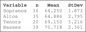
41. The summary statistics are shown here. Test, at α=0.01, whether the population mean heights of the groups differ.
12.1.41
Since the p-value≈ 0 is ≤0.01, we reject H0. There is evidence that not all the population mean heights are equal.
Nutritional Rating of Breakfast Cereals. Use this information for Exercises 42–45. Does the nutritional rating of breakfast cereals vary by manufacturer? The data set Breakfast Cereals 2 contains information on the nutritional rating and manufacturer for 68 breakfast cereals.4 Assume that the cereals were selected randomly from the manufacturers so that the selection of a cereal from one manufacturer did not affect the selection of cereals from other manufacturers.
Question 12.42
breakfastcereals2
42. What Result Might We Expect? The comparison boxplot of the nutritional ratings is shown here. Assume that the normality condition is satisfied.
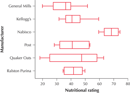
- Explain whether the plot may be considered evidence for or against the null hypothesis that all population mean nutritional ratings were equal.
- Would we expect the null hypothesis to be rejected or not to be rejected?
Question 12.43
breakfastcereals2
43. The largest standard deviation is SQuaker Oats=10.603, whereas the smallest is SNabisco=5.509. State whether the equal-variance requirement is satisfied.
12.1.43
Since SQuakerOats=10.603≤11.018=2 SNabisco, the equal variance requirement is satisfied.
Question 12.44
breakfastcereals2
44. Is the independence assumption validated? Why?
Question 12.45
breakfastcereals2
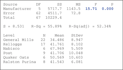
45. The Minitab output shown here contains the ANOVA results. Fdata and the p-value are in blue. Test, using level of significance α=0.05, whether all population mean nutritional ratings are equal across all manufacturers.
12.1.45
H0:μGeneralMills=μKelloggs=μNabisco=μPost=μQuakerOats=μRalstonPurina Ha: Not all the population means are equal. Reject H0 if the p-value≤0.05. Fdata=15.71; p-value≈ 0. Since the p-value is ≤0.05, we reject H0. There is evidence that the population mean nutritional ratings of the cereals made by the different manufacturers are not all equal.
Question 12.46
 46. Student-Run Café Business. Try to answer these questions without redoing the calculations and without rerunning the ANOVA. Refer to Exercise 31. What if more than 22 wraps were sold instead of the last entry for 22 recorded for the number of wraps sold?
- How would that change affect each entry in the ANOVA table?
- How would that change affect the conclusion, if at all?
Question 12.47
 47. Challenge Exercise: The professionals versus the Darts. Try to answer these questions without redoing the calculations and without rerunning the ANOVA. Refer to Exercise 32. What if we added three points to each value for the DJIA? (Hint: The sample mean for the DJIA is more than three points lower than the other two sample means.)
- How would that change affect each entry in the ANOVA table?
- How would that change affect the conclusion, if at all?
12.1.47
(a) (i) df1 and df2 would stay the same (ii) ˉˉx would increase (iii) SSTR would decrease (iv) SSE would stay the same (v) SST would decrease (vi) MSTR would decrease (vii) MSE would stay the same (viii) Fdata would decrease (ix) the p-value would increase. (b) Fdata would decrease and the p-value would increase. Therefore, the conclusion would still be do not reject H0.
BRINGING IT ALL TOGETHER
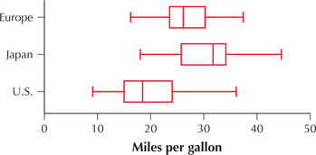
Gas Mileage for European, Japanese, and American Cars. Use this information for Exercises 48–50. The following figure shows a comparison boxplot of the vehicle mileage (in mpg) for random samples of automobiles manufactured in Europe, Japan, and the United States. The summary statistics are provided. We are interested in testing, using α=0.01, whether population mean gas mileage differs among automobiles from the three regions. Assume that the assumptions are satisfied.
| MPG | Sample 1: Europe |
Sample 2: Japan |
Sample 3: USA |
|---|---|---|---|
| Sample mean | ˉx1=27.603 | ˉx2=30.451 | ˉx3=20.033 |
| Sample standard deviation |
s1=6.58 | s2=6.09 | s3=6.440 |
| Sample size | n1=68 | n2=79 | n3=245 |
Question 12.48
48. What Result Might We Expect?
- Based on the graphical evidence in the comparison boxplot, what might be the conclusion? Explain your reasoning.
- Perform the ANOVA, using whichever method you prefer.
- Is your intuition from (a) supported?
Question 12.49
49. Confidence Intervals as Further Clues in ANOVA. Refer to Exercise 48. Suppose we construct a confidence interval for each of the population means. If at least one confidence interval does not overlap the others, then it is evidence against the null hypothesis.
- Use a t interval from Section 8.2 to construct a 99% confidence interval for the population mean gas mileage of
- European cars
- Japanese cars
- American cars
- Is there one confidence interval from (a) that does not overlap the other two? If so, what does this mean in terms of the null hypothesis that all the population means are equal?
12.1.49
(a) (i) (25.4805, 29.7255) (ii) (28.6366, 32.2654) (iii) (18.9526, 21.1134). (b) The confidence interval for the population mean gas mileage of American cars does not overlap the other two confidence intervals. This is evidence against the null hypothesis that all the population means are equal.
Question 12.50
 50. Refer to the table of descriptive summaries of vehicle mileage. What if we discovered that we made a mistake in the data collection and that every Japanese vehicle tested actually had 1 mpg higher gas mileage than previously recorded? Explain how and why this change would affect the following measures—increase, decrease, or no change.
- n
- k
- SSTR
- SSE
- SST
- MSTR
- MSE
- Fdata
- p-value
- Conclusion
WORKING WITH LARGE DATA SETS
For Exercises 51–54, use the Crash data set, which contains information about the severity of injuries sustained by crash dummies when the National Transportation Safety Board crashed automobiles into a wall at 35 miles per hour.
Question 12.51
crash
51. Head Injuries and Vehicle Size. The variable head_inj contains a measure of the severity of the head injury sustained by crash dummies. The variable size2 categorizes the type of vehicle, such as light, medium, heavy, pickup truck, MPV (SUV), and so on. The values of the variable size2 are as follows: 1 = compact car, 2 = light car, 3 = medium car, 4 = heavy car, = = minicompact car, 6 = van, 7 = pickup truck, and 8 = MPV (SUV). Would you expect the population mean severity of head injuries suffered by the dummies to be the same across all the size categories? Use technology to perform the analysis of variance, using α=0.05. Comment on the results.
12.1.51
H0:μ1=μ2=μ3=μ4=μ5=μ6=μ7=μ8.Ha: Not all the population means are equal. Reject H0 if the p-value≤0.05.8.27. p-value≈ 0. Since the p-value is ≤0.05, we reject H0. There is evidence that not all the population means are equal.

Question 12.52
crash
52. Head Injuries and Vehicle year. The variable year indicates the model year of the vehicle. Would you expect the population mean severity of head injuries suffered by the dummies to be the same across all model years? Use technology to perform the analysis of variance, using α=0.05. Comment on the results.
Question 12.53
crash
53. Chest Injury and protection Device. The variable chest_in is a measure of the severity of the chest injury suffered by the crash dummy. The variable protect2 categorizes the type of protection that the vehicle offers: 1 = manual seat belts, 2 = motorized seat belts, 3 = passive seat belts, 4 = dual air bags. Would you expect the population mean severity of chest injuries suffered by the dummies to be the same for all categories of protection? Use technology to perform the analysis of variance, using α=0.01. Comment on the results.
12.1.53
H0:μ1=μ2=μ3=μ4.Ha: Not all the population means are equal. Reject H0 if the p-value≤0.01.3.12. p-value= 0.026. Since the p-value is not ≤0.01, we do not reject H0. There is insufficient evidence that not all the population means are equal.

Question 12.54
crash
54. Refer to Exercise 53. Now use α=0.05. How does this affect your conclusion?
Question 12.55
55. Move the group means so that they are about the same by clicking and dragging the black dots so that they are about even horizontally.
- What happens to the value of F(Fdata)?
- Explain why this happens, using the concept of between-sample variability and the statistics SSTR, MSTR, and Fdata
12.1.55
(a) Decreases (b) Since all of the sample means are changed until they are about the same, SSTR and MSTR should decrease to small numbers. Since the variability of each sample stays the same, MSE stays the same. Thus Fdata=MSTRMSE decreases.
Question 12.56
56. Click Reset. Increase the Within-Sample Variability.
- What happens to the value of F(Fdata)?
- Explain why this change happens, using the concept of within-sample variability and the statistics SSE, MSE, and Fdata.
