13 Inference in Regression

13.2 Confidence Intervals and Prediction Intervals

OBJECTIVES By the end of this section, I will be able to …

Construct confidence intervals for the mean value of $y$ for a given value of $x$ .
Construct prediction intervals for a randomly chosen value of $y$ for a given value of $x$ .

1 Construct Confidence Intervals for the Mean Value of $y$ for a Given $x$

Suppose a cell phone company wants to increase sales to 20-year-olds, and therefore wants to estimate the number of text messages sent by 20-year-old men and women. In earlier sections, we learned how to calculate the predicted value $\hat{y}$ by using the regression equation $\hat{y} = b_{1} x + b_{0}$ For example, in Example 1 (page 716), we saw that the predicted number of text messages for the 20-year-old texter is $\hat{y} = (- 1.5) (20) + 60.6 = 30.6$ messages. However, this estimate of 30.6 messages is only a point estimate, similar to using the sample mean $\bar{x}$ alone to estimate the unknown population mean $μ$ . We learned in Section 8.1 about the pitfalls of point estimates, such as the lack of a measure of confidence associated with the estimate. So, just as we learned about confidence intervals for $μ$ in Chapter 8, in this section we will learn how to construct:

confidence intervals for the mean value of $y$ for a given value of $x$ , and
prediction intervals for a randomly chosen value of $y$ for a given value of $x$ .

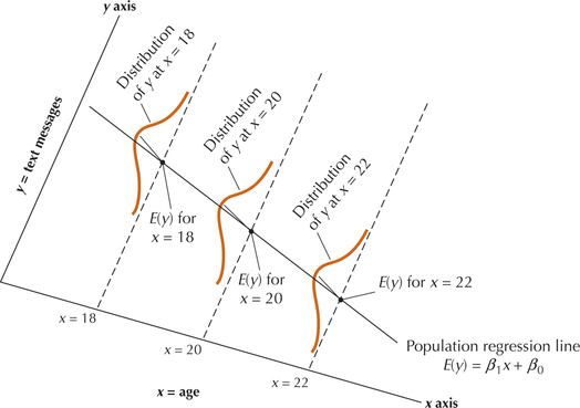
Refer to Figure 3 (reproduced here from page 719), which illustrates the regression assumptions. Note that, for $x = 20$ , there is assumed to be an entire population of $y$ -values. The cell phone company is interested in this population, and wants to construct a confidence interval for the mean number of text message sent by all 20-year-olds.

FIGURE 3 For

$x = 20$ years old, there is an entire population of

$y = number of text messages$ .

Page 738

Confidence Interval for the Mean Value of $y$ for a Given $x$ A $100 (1 - α) %$ confidence interval for the mean response, that is, for the population mean of all values of $y$ , given a value of $x$ , may be constructed using the following lower and upper bounds:

$\begin{matrix} Lower bound : \hat{y} - t_{α / 2} . s \sqrt{\frac{1}{n} + \frac{{(x * - \bar{x})}^{2}}{\sum {(x_{i} - \bar{x})}^{2}}} \\ Upper bound : \hat{y} + t_{α / 2} . s \sqrt{\frac{1}{n} + \frac{{(x * - \bar{x})}^{2}}{\sum {(x_{i} - \bar{x})}^{2}}} \end{matrix}$

where $x *$ represents the given value of the predictor variable $x$ , $s = \sqrt{\frac{MSE}{n - 2}}$ represents the standard error of the estimate, $n$ is the number of observations, $\bar{x}$ is the sample mean of the $x$ -values, and $t_{α / 2}$ is the critical value with $n - 2$ degrees of freedom. The requirements for the confidence interval are met if the regression assumptions are met.

Let's look at an example of constructing and interpreting such a confidence interval

EXAMPLE 8 Constructing and interpreting a confidence interval for the mean value of $y$ for a given $x$

Construct and interpret a 95% confidence interval for the population mean number of text messages sent for all 20-year-olds.

Solution

Example 2 showed that the regression assumptions for this data set are met, thus allowing us to construct this confidence interval.

Using our given value $x * = 20$ , we calculate the point estimate as follows: $\hat{y} = (- 1.5) (20) + 60.6 = 30.6$ .
The data set in Table 1 shows that there are $n = 10$ people, so that the degrees of freedom for the $t$ critical value is $n - 2 = 8$ . From the $t$ table (Table D in the Appendix), the $t$ critical value for confidence level 95% is $t_{α / 2} = 2.306$ .
In Example 3, we calculated $\sum {(x - \bar{x})}^{2} = 330$ and the standard error of the estimate to be $s \approx 2.4083$ .
The Minitab output in Figure 17 shows that $\bar{x} = 27$ years of age.

FIGURE 17 Minitab shows $\bar{x} = 27$ .

Thus,

$\begin{array}{l} Lower bound: & \hat{y} - t_{α / 2} \cdot s \sqrt{\frac{1}{n} + \frac{{(x^{*} - \bar{x})}^{2}}{{\sum (x_{i} - \bar{x})}^{2}}} \\ \approx 30.6 - (2.306) \cdot 2.4083 \sqrt{\frac{1}{10} + \frac{{(20 - 27)}^{2}}{330}} \approx 27.8317 \\ Upper bound: & \hat{y} + t_{α / 2} \cdot s \sqrt{\frac{1}{n} + \frac{{(x^{*} - \bar{x})}^{2}}{{\sum (x_{i} - \bar{x})}^{2}}} \\ \approx 30.6 + (2.306) \cdot 2.4083 \sqrt{\frac{1}{10} + \frac{{(20 - 27)}^{2}}{330}} \approx 33.3683 \end{array}$

We are 95% confident that the number of text messages sent by a randomly selected 20-year-old lies between 24.3947 and 36.8053.

Extrapolation (page 215) continues to be a danger for confidence intervals and prediction intervals. For example, it would not have been wise to ask for a confidence interval for the population mean number of text messages sent by all 50-year-old people because $x = 50$ lies outside the range of $x$ .

NOW YOU CAN DO

Exercises 3–8.

Page 739

2 Construct Prediction Intervals for an Individual Value of $y$ for a Given $x$

The formula for constructing a prediction interval for an individual random value of $y$ is similar to that for the confidence interval for the mean $y$ , except that the margin of error is larger. We talk about why this is so later in this section.

Prediction Interval for a Randomly Selected Value of $y$ for a Given $x$

A $100 (1 - α) %$ prediction interval for a randomly selected value of $y$ given a value of $x$ may be constructed using the following lower and upper bounds:

$\begin{matrix} Lower bound : \hat{y} - t_{α / 2} \cdot s \sqrt{1 + \frac{1}{n} + \frac{{(x^{*} - \bar{x})}^{2}}{\sum {(x_{i} - \bar{x})}^{2}}} \\ Upper bound : \hat{y} + t_{α / 2} \cdot s \sqrt{1 + \frac{1}{n} + \frac{{(x^{*} - \bar{x})}^{2}}{\sum {(x_{i} - \bar{x})}^{2}}} \end{matrix}$

where $x^{*}$ represents the given value of the predictor variable $x$ , $s = \sqrt{\frac{MSE}{n - 2}}$ represents the standard error of the estimate, $n$ is the number of observations, $\bar{x}$ is the sample mean of the $x$ values, and $t_{α / 2}$ is the critical value with $n - 2$ degrees of freedom. The requirements for the confidence interval are met if the regression assumptions are met.

EXAMPLE 9 Constructing and interpreting a prediction interval for a randomly selected value of $y$ for a given $x$

Construct and interpret a 95% prediction interval for the number of text messages sent by a randomly selected 20-year-old.

Solution

The requirements for the prediction interval are the same as for the confidence interval, so we know from Example 8 that the requirements for constructing the prediction interval are met. Using the values obtained in Example 8, we calculate the lower and upper bounds as follows:

$\begin{array}{l} Lower bound: & \hat{y} - t_{α / 2} \cdot s \sqrt{1 + \frac{1}{n} + \frac{{(x^{*} - \bar{x})}^{2}}{{\sum (x_{i} - \bar{x})}^{2}}} \\ \approx 30.6 - (2.306) \cdot 2.4083 \sqrt{1 + \frac{1}{10} + \frac{{(20 - 27)}^{2}}{330}} \approx 24.3947 \\ Upper bound: & \hat{y} + t_{α / 2} \cdot s \sqrt{1 + \frac{1}{n} + \frac{{(x^{*} - \bar{x})}^{2}}{{\sum (x_{i} - \bar{x})}^{2}}} \\ \approx 30.6 + (2.306) \cdot 2.4083 \sqrt{1 + \frac{1}{10} + \frac{{(20 - 27)}^{2}}{330}} \approx 36.8053 \end{array}$

We are 95% confident that the number of text messages sent by a randomly selected 20-year-old lies between 24.3947 and 36.8053.

NOW YOU CAN DO

Exercises 9–14.

Page 740

Developing Your Statistical Sense

Why Are Prediction Intervals Wider?

The prediction interval (24.3947, 36.8053) from Example 9 is wider than the corresponding confidence interval from Example 8. This is true in general, but why? Note that the only difference in the formulas for the prediction interval, compared to the confidence interval, is the “1 +” inside the radical in the formula for the prediction interval. This ensures that the prediction interval always has a larger margin of error than the confidence interval for a given $x$ . This larger margin of error reflects the greater variability of individual responses compared to the mean response.

To see how individual values have greater variability than their means, consider that you would probably stand a better chance of guessing the class mean height to within 2 inches instead of the height of a randomly chosen student. This is because the variability of the randomly selected $y$ is larger than that of the mean $y$ . In the one-sample case, this is because the standard deviation $σ$ of a particular value of $x$ is always larger than the standard deviation of the sample mean $\bar{x}$ , which is $σ_{\bar{x}} = σ / \sqrt{n}$ . Similarly, the prediction interval for a randomly chosen $y$ is wider than the confidence interval for the mean value of $y$ , for a given value of $x$ .

Finally, we illustrate the use of technology to construct confidence intervals and prediction intervals.

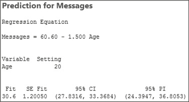
EXAMPLE 10 Confidence intervals and prediction intervals using technology

Use Minitab and JMP to construct a 95% confidence interval for the population mean number of text messages sent by all 20-year-olds, and to construct a 95% prediction interval for the number of text messages sent by a randomly selected 20-year-old.

Solution

We use the instructions provided in the Step-by-Step Technology Guide below. Figure 18 shows the Minitab results, and Figure 19 shows the JMP results.

FIGURE 18 Minitab results for confidence interval and prediction interval.

FIGURE 19 JMP results for confidence interval and prediction interval.