9 Hypothesis Testing

Section 9.3 Exercises

CLARIFYING THE CONCEPTS

Question 9.107

1. True or false: It is possible to get a $p$ -value equal to 1.5. (p. 508)

9.3.1

False

Question 9.108

2. State the rejection rule for the $p$ -value method for performing the Z test for μ. (p. 509)

Question 9.109

3. Explain why we might want to assess the strength of evidence against the null hypothesis, instead of delivering a simple “reject $H_{0}$ or do not reject $H_{0}$ ” conclusion. (p. 514)

9.3.3

It gives us extra information about whether $H_{0}$ was barely rejected or not rejected or whether it was a no-brainer decision to reject or not reject $H_{0}$ .

Page 521

Question 9.110

4. What is the criterion for rejecting $H_{0}$ when using a confidence interval to perform a two-tailed hypothesis test for $μ$ ? (p. 517)

Question 9.111

5. True or false: For a right-tailed test, when $Z_{data} < Z_{crit}$ , the $p$ -value is always < $α$ . (p. 516)

9.3.5

False

Question 9.112

6. For (a)–(c), indicate whether or not the quantity represents a probability. (p. 516)

$Z_{data}$
$p$ -value
$α$

PRACTICING THE TECHNIQUES

CHECK IT OUT!

To do	Check out	Topic
Exercises 7–20	Example 12	Calculating the $p$ -value
Exercises 21–26	Example 13	One-tailed $Z$ test for $μ$
Exercises 27–30	Example 14	Two-tailed $Z$ test for $μ$
Exercises 31–40	Example 15	Assessing the strength of evidence against $H_{0}$
Exercises 41–46	Example 16	Equivalence of two-tailed tests and confidence intervals
Exercises 47–50	Example 17	Interpreting software output

For Exercises 7–40, assume that the conditions for performing the $Z$ test are met.

For Exercises 7–17, find the $p$ -value.

Question 9.113

7. $H_{0} : μ = 10 vs . H_{a} : μ > 10, Z_{data} = 1.5$

9.3.7

0.0668

Question 9.114

8. $H_{0} : μ = 10 vs . H_{a} : μ > 10, Z_{data} = 2.5$

Question 9.115

9. $H_{0} : μ = 25 vs . H_{a} : μ > 25, Z_{data} = 0.6$

9.3.9

0.2743

Question 9.116

10. $H_{0} : μ = 25 vs . H_{a} : μ > 25, Z_{data} = 1.2$

Question 9.117

11. $H_{0} : μ = 200 vs . H_{a} : μ < 200, Z_{data} = - 0.7$

9.3.11

0.2420

Question 9.118

12. $H_{0} : μ = 200 vs . H_{a} : μ < 200, Z_{data} = - 1.27$

Question 9.119

13. $H_{0} : μ = 69 vs . H_{a} : μ < 69, Z_{data} = - 2.23$

9.3.13

0.0129

Question 9.120

14. $H_{0} : μ = 69 vs . H_{a} : μ < 69, Z_{data} = - 2.55$

Question 9.121

15. $H_{0} : μ = 31 vs . H_{a} : μ \neq 31, Z_{data} = 0.64$

9.3.15

0.5222

Question 9.122

16. $H_{0} : μ = 31 vs . H_{a} : μ \neq 31, Z_{data} = - 0.64$

Question 9.123

17. $H_{0} : μ = 12 vs . H_{a} : μ \neq 12, Z_{data} = 0$

9.3.17

Question 9.124

18. Refer to Exercises 7–10. Explain what happens to the $p$ -value for a right-tailed test as $Z_{data}$ moves toward the right tail.

Question 9.125

19. Refer to Exercises 11–14. Explain what happens to the $p$ -value for a left-tailed test as $Z_{data}$ moves toward the left tail.

9.3.19

It decreases.

Question 9.126

20. Refer to Exercises 15 and 16. What can we say about the $p$ -values of two two-tailed tests whose values of $Z_{data}$ have the same absolute value?

For Exercises 21–30, perform the $Z$ test for $μ$ using level of significance a $α = 0.05$ by doing the following steps:

State the hypotheses and the rejection rule.
Calculate $Z_{data}$ .
Find the $p$ -value.
State the conclusion and the interpretation.

Question 9.127

21. $H_{0} : μ = 3.14 vs . H_{a} : μ > 3.14, \bar{x} = 3.2, σ = 1, n = 100$

9.3.21

(a) $H_{0} : μ = 3.14 vs . H_{a} : μ > 3.14$ . We will reject $H_{0}$ if the $p -value \leq α = 0.05$ . (b) $Z_{data} = 0.6$ (c) $p -value = 0.2743$ (d) The $p -value = 0.2743$ is not $\leq 0.05$ . Therefore we do not reject $H_{0}$ . There is insufficient evidence at level of significance $α = 0.05$ that the population mean is greater than 3.14.

Question 9.128

22. $H_{0} : μ = 30 vs . H_{a} : μ < 30, \bar{x} = 25, σ = 10, n = 16$

Question 9.129

23. $H_{0} : μ = - 1.0 vs . H_{a} : μ > - 1.0, \bar{x} = 0, σ = 1, n = 400$

9.3.23

(a) $H_{0} : μ = - 1.0 vs . H_{a} : μ > - 1.0$ We will reject $H_{0}$ if the $p -value \leq α = 0.05$ . (b) $Z_{data} = 20$ (c) $p - v \approx 0$ (d) The $p -value \approx 0.2743$ is $\leq 0.05$ . Therefore we reject $H_{0}$ . There is evidence at level of significance $α = 0.05$ that the population mean is greater than -1.0.

Question 9.130

24. $H_{0} : μ = 2000 vs . H_{a} : μ > 2000, \bar{x} = 2050, σ = 200, n = 25$

Question 9.131

25. $H_{0} : μ = 500 vs . H_{a} : μ < 500, \bar{x} = 450, σ = 100, n = 16$

9.3.25

(a) $H_{0} : μ = 500 vs . H_{a} : μ < 500$ . We will reject $H_{0}$ if the $p -value \leq α = 0.05$ . (b) $Z_{data} = - 2$ (c) $p -value = 0.0228$ (d) The $p -value = 0.0228$ is $\leq 0.05$ . Therefore we reject $H_{0}$ . There is evidence at level of significance $α = 0.05$ that the population mean is less than 500.

Question 9.132

26. $H_{0} : μ = - 32 vs . H_{a} : μ > - 32, \bar{x} = - 30, σ = 40, n = 400$

Question 9.133

27. $H_{0} : μ = 10 vs . H_{a} : μ \neq 10, \bar{x} = 10, σ = 5, n = 100$

9.3.27

(a) $H_{0} : μ = 10 vs . H_{a} : μ \neq 10$ . We will reject $H_{0}$ if the $p -value \leq α = 0.05$ . (b) $Z_{data} = 0$ (c) $p -value = 1$ (d) The $p -value = 1$ is not $\leq 0.05$ . Therefore we do not reject $H_{0}$ . There is insufficient evidence at level of significance $α = 0.05$ that the population mean is not equal to 10.

Question 9.134

28. $H_{0} : μ = - 5 vs . H_{a} : μ \neq - 5, \bar{x} = - 5, σ = 1.5, n = 100$

Question 9.135

29. $H_{0} : μ = 0 vs . H_{a} : μ \neq 0, \bar{x} = - 0.12, σ = 0.4, n = 81$

9.3.29

(a) $H_{0} : μ = 0 vs . H_{a} : μ \neq 0$ . We will reject $H_{0}$ if the $p -value \leq α = 0.05$ .

(b) $Z_{data} = - 2.7$ (c) $p -value = 0.0070$ (d) The $p -value = 0.0070$ is $\leq 0.05$ . Therefore we reject $H_{0}$ . There is evidence at level of significance $α = 0.05$ that the population mean is not equal to 0.

Question 9.136

30. $H_{0} : μ = 46 vs . H_{a} : μ \neq 46, \bar{x} = 47, σ = 15, n = 225$

For Exercises 31–40, use the indicated $p$ -value to assess the strength of evidence against the null hypothesis, using Table 6.

Question 9.137

31. $p$ -value from Exercise 21

9.3.31

The $p -value$ of 0.2743 implies that there is no evidence against the null hypothesis that the population mean equals 3.14.

Question 9.138

32. $p$ -value from Exercise 22

Question 9.139

33. $p$ -value from Exercise 23

9.3.33

The $p -value$ of approximately 0 implies that there is extremely strong evidence against the null hypothesis that the population mean equals −1.0.

Question 9.140

34. $p$ -value from Exercise 24

Question 9.141

35. $p$ -value from Exercise 25

9.3.35

The $p -value$ of 0.0228 implies that there is solid evidence against the null hypothesis that the population mean equals 500.

Question 9.142

36. $p$ -value from Exercise 26

Question 9.143

37. $p$ -value from Exercise 27

9.3.37

The $p -value$ of 1 implies that there is no evidence against the null hypothesis that the population mean equals 10.

Question 9.144

38. $p$ -value from Exercise 28

Question 9.145

39. $p$ -value from Exercise 29

9.3.39

The $p -value$ of 0.007 implies that there is very strong evidence against the null hypothesis that the population mean equals 0.

Question 9.146

40. $p$ -value from Exercise 30

For Exercises 41–46, a $100 (1 - α) %$ $Z$ confidence interval is given (see Section 8.1). Use the confidence interval to test, using level of significance $α$ , whether $μ$ differs from each of the indicated hypothesized values.

Question 9.147

41. A 95% $Z$ confidence interval for $μ$ is (−2.7, 6.9). Hypothesized values $μ_{0}$ are

−3
−2
0
5
7

9.3.41

	Value of $μ_{o}$	Form of hypothesis test, with $α - 0.05$	Where $μ_{o}$ lies in relation to 95% confidence interval	Conclusion of hypothesis test
a.	–3	$H_{0} : μ = - 3 vs . H_{a} : μ \neq - 3$	Outside	Reject $H_{0}$
b.	−2	$H_{0} : μ = - 2 vs . H_{a} : μ \neq - 2$	Inside	Do not reject $H_{0}$
c.	0	$H_{0} : μ = 0 vs . H_{a} : μ \neq 0$	Inside	Do not reject $H_{0}$
d.	5	$H_{0} : μ = 5 vs . H_{a} : μ \neq 5$	Inside	Do not reject $H_{0}$
e.	7	$H_{0} : μ = 7 vs . H_{a} : μ \neq 7$	Outside	Reject $H_{0}$

Question 9.148

42. A 99% $Z$ confidence interval for $μ$ is (45, 55). Hypothesized values $μ_{0}$ are

Question 9.149

43. A 90% $Z$ confidence interval for $μ$ is (−10, −5). Hypothesized values $μ_{0}$ are

−3
−8
−11
0
7

9.3.43

	Value of $μ_{o}$	Form of hypothesis test, with $α = 0.10$	Where $μ_{o}$ lies in relation to 90% confidence interval	Conclusion of hypothesis test
a.	–3	$H_{0} : μ = - 3 vs . H_{a} : μ \neq - 3$	Outside	Reject $H_{0}$
b.	–8	$H_{0} : μ = - 8 vs . H_{a} : μ \neq - 8$	Inside	Do not reject $H_{0}$
c.	–11	$H_{0} : μ = - 11 vs . H_{a} : μ \neq - 11$	Outside	Reject $H_{0}$
d.	0	$H_{0} : μ = 0 vs . H_{a} : μ \neq 0$	Outside	Reject $H_{0}$
e.	7	$H_{0} : μ = 7 vs . H_{a} : μ \neq 7$	Outside	Reject $H_{0}$

Question 9.150

44. A 95% $Z$ confidence interval for $μ$ is (1024, 2056). Hypothesized values $μ_{0}$ are

1000
2000
3000
0
1025

Question 9.151

45. A 95% $Z$ confidence interval for $μ$ is (0, 1). Hypothesized values $μ_{0}$ are

1.5
−1
0.5
0.9
1.2

9.3.45

	Value of $μ_{o}$	Form of hypothesis test, with $α = 0.05$	Where $μ_{o}$ lies in relation to 95% confidence interval	Conclusion of hypothesis test
a.	1.5	$H_{0} : μ = 1.5 vs . H_{a} : μ \neq 1.5$	Outside	Reject $H_{0}$
b.	–1	$H_{0} : μ = - 1 vs . H_{a} : μ \neq - 1$	Outside	Reject $H_{0}$
c.	0.5	$H_{0} : μ = 0.5 vs . H_{a} : μ \neq 0.5$	Inside	Do not reject $H_{0}$
d.	0.9	$H_{0} : μ = 0.9 vs . H_{a} : μ \neq 0.9$	Inside	Do not reject $H_{0}$
e.	1.2	$H_{0} : μ = 1.2 vs . H_{a} : μ \neq 1.2$	Outside	Reject $H_{0}$

Question 9.152

46. A 95% $Z$ confidence interval for $μ$ is (1.3275, 1.4339). Hypothesized values $μ_{0}$ are

1.3
1.35
1.4
1.45
1.3275

For Exercises 47–50, software output from a $Z$ test for $μ$ is provided. For each, examine the indicated software output, and provide the following steps for level of significance $α = 0.05$ :

Step 1 State the hypotheses and the rejection rule.
Step 2 Find $Z_{data}$ .
Step 3 Find the $p$ -value.
Step 4 State the conclusion and interpretation.

Page 522

Question 9.153

47.

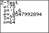
9.3.47

Step 1 $H_{0} : μ = 75 vs . H_{a} : μ < 75$

We will reject $H_{0}$ if the $p -value \leq α = 0.05$ .

Step 2 $Z_{data} = - 1.6$

Step 3 $p -value = 0 .0547992894$

Step 4 The $p -value = 0.0547992894$ is not $\leq 0.05$ . Therefore we do not reject $H_{0}$ . There is insufficient evidence at level of significance $α = 0.05$ that the population mean is less than 75.

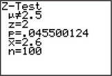
Question 9.154

48.

Question 9.155

49.

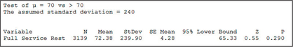
9.3.49

Step 1 $H_{0} : μ = 70 vs . H_{a} : μ > 70$

We will reject $H_{0}$ if the $p -value \leq α = 0.05$ .

Step 2 $Z_{data} = 0.55$

Step 3 $p -value = 0. 290$

Step 4 The $p -value = 0. 290$ is not $\leq 0.05$ . Therefore we do not reject $H_{0}$ . There is insufficient evidence at level of significance $α = 0.05$ that the population mean is greater than 70.

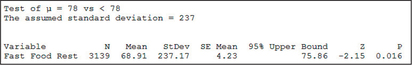
Question 9.156

50.

APPLYING THE CONCEPTS

For Exercises 51–58, do the following:

State the hypotheses and the rejection rule.
Calculate $Z_{data}$ .
Find the $p$ -value.
State the conclusion and the interpretation.

Question 9.157

51. Car Insurance. Like sports cars? They can be expensive. Time.com/Money reports that in 2014 the mean annual car insurance premium for a Porsche Panamera Turbo-S was $3000. Suppose that a random sample of nine such Porsches taken this year has a mean car insurance premium of $3120. Assume $σ = $ 600$ , and assume that the distribution of premiums is normal. Test whether the population mean premium has increased, using level of significance $α = 0.10$ .

9.3.51

(a) $H_{0} : μ = 3000 vs . H_{a} : μ > 3000$ . We will reject $H_{0}$ if the $p -value \leq α = 0.10$ . (b) $Z_{data} = 0.6$ (c) $p -value = 0.2743$ (d) The $p -value = 0. 2743$ is not $\leq 0.10$ . Therefore we do not reject $H_{0}$ . There is insufficient evidence at level of significance $α = 0.10$ that the population mean annual car insurance premium for a Porsche Panamera Turbo-S has increased from $3000.

Question 9.158

52. Mobile Apps. In 2014, Nielsen reported that young people ages 18–24 spent 37 hours per month using the apps on their mobile devices. Suppose that a random sample of 100 people ages 18–24 showed a sample mean of 40 hours. Assume $σ = 20$ . Test whether the population mean number of hours using mobile apps by young people ages 18–24 has increased, at level of significance $α = 0.05$ .

Question 9.159

53. Eating Trends. According to an NPD Group report, the mean number of meals prepared and eaten at home is less than 700 per year. Suppose that a random sample of 100 households showed a sample mean number of meals prepared and eaten at home of 650. Assume $σ = 25$ . Test whether the population mean number of such meals is less than 700, using level of significance $α = 0.10$ .

9.3.53

(a) $H_{0} : μ = 700 vs . H_{a} : μ < 700$ . Reject $H_{0}$ if the $p -value \leq 0.10$ .

(b) −20 (c) $\approx 0$ (d) Since the $p -value \leq α$ , reject $H_{0}$ . There is evidence that the population mean number of meals prepared and eaten at home is less than 700.

Question 9.160

54. DDT in Breast Milk. Researchers compared the amount of DDT in the breast milk of 12 Latina women in the Yakima Valley of Washington State with the amount of DDT in breast milk in the general U.S. population.³ They measured the mean DDT level in the general population to be 47.2 parts per billion (ppb) and the mean DDT level in the 12 Latina women to be 219.7 ppb. Assume $σ = 36$ and a normally distributed population. Test whether the population mean DDT level in the breast milk of Latina women in the Yakima Valley is greater than that of the general population, using level of significance a $σ = 0.01$ .

Question 9.161

55. Millennials' Income. The Pew Research Center reported in 2014 that Millennials (those ages 25–32) with Bachelor's degrees working full time are making on average $17,500 more per year than those Millennials with only a high school education ($45,500 vs. $28,000). Suppose that, in a random sample of 36 Millennials with Bachelor's degrees taken today, the sample mean income is $50,000. Assume $σ = $ 18, 000$ . Test whether the population mean annual income has increased from its previous value of $45,500 using level of significance $α = 0.05$ .

9.3.55

(a) $H_{0} : μ = 45,500 vs . H_{a} : μ > 45,500$ . We will reject $H_{0}$ if the $p -value \leq α = 0.05$ . (b) $Z_{data} = 1.5$ (c) $p -value = 0.0668$ (d) The $p -value = 0. 0668$ is not $\leq 0.05$ . Therefore we do not reject $H_{0}$ . There is insufficient evidence at level of significance $α = 0.05$ that the population mean annual income of Millennials with Bachelor's degrees working full time has increased from $45,500.

Question 9.162

56. Tree Rings. Do trees grow more quickly when they are young? The International Tree Ring Data Base collected data on a particular 440-year-old Douglas fir tree.⁴ The mean annual ring growth in the tree's first 80 years of life was 1.4261 millimeters (mm). A random sample of size 100 taken from the tree's later years showed a sample mean growth of 0.56 mm per year. Assume $σ = 0.5 mm$ and a normally distributed population. Test whether the population mean annual ring growth in the tree's later years is less than 1.4261 mm, using level of significance $α = 0.05$ .

Question 9.163

57. Hybrid Vehicles. A study by Edmunds.com examined the time it takes for owners of hybrid vehicles to recoup their additional initial cost through reduced fuel consumption. Suppose that a random sample of nine hybrid cars showed a sample mean time of 2.1 years. Assume that the population is normal with $σ = 0.2$ . Test, using level of significance $α = 0.01$ , whether the population mean time it takes owners of hybrid cars to recoup their initial cost is less than three years.

9.3.57

(a) $H_{0} : μ = 3 vs . H_{a} : μ < 3$ . Reject $H_{0}$ if the $p -value \leq 0. 01$ . (b) −13.5 (c) $p -value \approx 0$ (d) Since the $p -value \leq α$ , reject $H_{0}$ . There is evidence that the population mean time hybrid cars take to recoup their initial cost is less than 3 years.

Question 9.164

58. Americans' Height. Americans used to be, on average, the tallest people in the world. That is no longer the case, according to a study by Dr. Richard Steckel, professor of economics and anthropology at The Ohio State University. The Norwegians and Dutch are now the tallest, at 178 centimeters, followed by the Swedes at 177, and then the Americans, with a mean height of 175 centimeters (approximately 5 feet 9 inches). According to Dr. Steckel, “The average height of Americans has been pretty much stagnant for 25 years.”⁵ Suppose a random sample of 100 Americans taken this year shows a mean height of 174 centimeters, and we assume $σ = 10 centimeters$ . Test, using level of significance $α = 0.01$ , whether the population mean height of Americans this year has changed from 175 centimeters.

For Exercises 59–66, use the $p$ -value from the indicated exercise to assess the strength of evidence against the null hypothesis, using Table 6.

Question 9.165

59. Car Insurance. Exercise 51.

9.3.59

The $p -value$ of 0.2743 implies that there is no evidence against the null hypothesis that the population mean equals $3000.

Question 9.166

60. Mobile Apps. Exercise 52.

Question 9.167

61. Eating Trends. Exercise 53.

9.3.61

The $p -value$ of approximately 0 implies that there is extremely strong evidence against the null hypothesis that the population mean equals 700 meals.

Question 9.168

62. DDT in Breast Milk. Exercise 54.

Question 9.169

63. Millennials' Income. Exercise 55.

9.3.63

The $p -value$ of 0.0668 implies that there is moderate evidence against the null hypothesis that the population mean equals $45,500.

Question 9.170

64. Tree Rings. Exercise 56.

Question 9.171

65. Hybrid Vehicles. Exercise 57.

9.3.65

The $p -value$ of approximately 0 implies that there is extremely strong evidence against the null hypothesis that the population mean equals 3 years.

Question 9.172

66. Americans' Height. Exercise 58.

Question 9.173

67. Advanced Placement Californians. The College Board reports that the mean score on all advanced placement tests taken in California in 2012 was 2.95. Suppose that a random sample of 49 test scores for tests taken by Californians this year is 2.95. Assume the population standard deviation is 0.21.

Page 523

Construct a 95% $Z$ confidence interval for the population mean test score for this year. (Hint: See Section 8.1.)
Use the confidence interval to test, at level of significance $α = 0.05$ , whether the population mean test score differs from the following amounts:
1. 2.89
2. 2.90
3. 3.00
4. 3.01

9.3.67

(a) (2.89, 3.01)

(b)

	Value of $μ_{o}$	Form of hypothesis test, with $α = 0.05$	Where $μ_{0}$ lies in relation to 95% confidence interval	Conclusion of hypothesis test
(i)	2.89	$H_{0} : μ = 2.89 vs . H_{a} : μ \neq 2.89$	Outside	Reject $H_{0}$
(ii)	2.90	$H_{0} : μ = 2.90 vs . H_{a} : μ \neq 2.90$	Inside	Do not reject $H_{0}$
(iii)	3.00	$H_{0} : μ = 3.00 vs . H_{a} : μ \neq 3.00$	Inside	Do not reject $H_{0}$
(iv)	3.01	$H_{0} : μ = 3.01 vs . H_{a} : μ \neq 3.01$	Outside	Reject $H_{0}$

Question 9.174

68. Engineers' Starting Salary. The National Association of Colleges and Employers reported in 2013 that the college major with the highest mean starting salary was engineering, with $62,600. Suppose that a random sample of 36 engineering starting salaries is $62,600. Assume the population standard deviation is $10,000.

Construct a 99% Z confidence interval for the population mean starting salary for engineers. (Hint: See Section 8.1.)
Use the confidence interval to test, at level of significance $α = 0.01$ , whether the population mean starting salary for engineers differs from the following amounts:
1. $66,000
2. $58,000
3. $67,000
4. $59,000

Health Care Premiums. Use the following information for Exercises 69–71. The National Conference of State Legislatures reports that the mean annual premium for employer-sponsored family health insurance coverage was $16,351 in 2014. A random sample of 100 such families showed a mean annual premium of $17,251. Assume $σ = $ 5000$ .

Question 9.175

69. Test whether the population mean annual premium is greater than $16,351, using level of significance $α = 0.05$ .

9.3.69

$H_{0} : μ = 16, 351 vs . H_{a} : μ > 16, 351$ . We will reject $H_{0}$ if the $p -value \leq α = 0.05$ . $Z_{data} = 1.8$ . $p -value = 0.0359$ . The $p -value = 0.0359$ is $\leq 0.05$ . Therefore we reject $H_{0}$ . There is evidence at level of significance $α = 0.05$ that the population mean annual premium for employer-sponsored family health insurance coverage has increased from $16,351.

Question 9.176

70. What if the sample mean premium equaled some value larger than $17,251, while everything else stayed the same? Explain how this change would affect the following, if at all:

The hypotheses
$Z_{crit}$
The critical region
$Z_{data}$
The conclusion

Question 9.177

71. Test whether the population mean annual premium is greater than $16,351 using level of significance $α = 0.01$ . Compare your conclusion with the conclusion in Exercise 70. Suggest two possible methods to resolve this contradiction.

9.3.71

$H_{0} : μ = 16, 351 vs . H_{a} : μ > 16, 351$ . We will reject $H_{0}$ if the $p -value \leq α = 0.01$ . $Z_{data} = 1.8$ . $p -value = 0.0359$ . The $p -value = 0.0359$ is not $\leq 0.01$ . Therefore we do not reject $H_{0}$ . There is insufficient evidence at level of significance $α = 0.01$ that the population mean annual premium for employer-sponsored family health insurance coverage has increased from $16,351. Turn to a direct assessment of the strength of evidence against the null hypothesis or obtain more data.

Mean Family Size. Use the following information for Exercises 72–74: According to the Statistical Abstract of the United States, the mean family size in 2010 was 3.14 persons, reflecting a slow decrease since 1980, when the mean family size was 3.29 persons. Has this trend continued to the present day? Suppose a random sample of 225 families taken this year yields a sample mean size of 3.05 persons, and suppose we assume that the population standard deviation of family sizes is 1 person.

Question 9.178

72. Test whether the population mean family size in America has decreased since 2010, using the $p$ -value method and level of significance $α = 0.05$ . (Try using the $p$ -value applet to help you solve this problem.)

Question 9.179

73. Refer to Exercise 72.

What is the smallest $p$ -value for which you will reject $H_{0}$ ?
Which type of error is it possible that we are making—a Type I error or a Type II error? Which type of error are we certain we are not making?
Suppose a newspaper headline referring to the study was “Mean Family Size Decreasing.” Is the headline supported or not supported by the data and the hypothesis test?

9.3.73

(a) 0 (b) Type II error; Type I error (c) This headline is not supported by the data and our hypothesis test.

Question 9.180

74. Refer to Exercises 72 and 73, What if the 3.05 persons had been a typo, and the actual sample mean was 3.00 persons? How would this have affected the following?

$Z_{data}$
The $p$ -value
The conclusion

Question 9.181

75. Women's Heart Rates. A random sample of 15 women produced the normal probability plot for their heart rates shown here. The sample mean was 75.6 beats per minute. Suppose the population standard deviation is known to be 9.

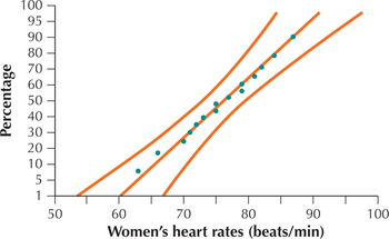
Discuss the evidence for or against the normality assumption. Should we use the $Z$ test? Why or why not?
Assume that the plot does not contradict the normality assumption; test whether the population mean heart rate for all women is less than 78, using level of significance $α = 0.05$ .
Test whether the population mean heart rate for all women differs from 78, using $α = 0.05$ .

9.3.75

(a) Yes, the normal probability plot indicates acceptable normality. (b) $H_{0} : μ = 78 vs . H_{a} : μ < 78$ . Reject $H_{0}$ if $p -value \leq 0.05$ , $Z_{data} = - 1.03$ , $p -value = 0.1515$ . Since $p -value = 0.1515$ is not $\leq α = 0.05$ , do not reject $H_{0}$ . There is insufficient evidence at level of significance $α = 0.05$ that the population mean heart rate for all women is less than 78 beats per minute.

(c) $H_{0} : μ = 78 vs . H_{a} : μ \neq 78$ . Reject $H_{0}$ if $p -value \leq 0.05$ . $Z_{data} = - 1.03$ . $p -value = 0.303$ . Since $p -value = 0.303$ is not $\leq α = 0.05$ , do not reject $H_{0}$ . There is insufficient evidence that the population mean heart rate for all women is different from 78 beats per minute.

Question 9.182

76. Challenge Exercise. Refer to the previous exercise.

Compare your conclusions from Exercises 75(b) and 75(c). Note that the conclusions differ, but the meanings of the hypotheses tested also differ. Combine the two conclusions into a single sentence. Do you find this sentence difficult to explain?
Explain in your own words the difference between the hypotheses in Exercises 75(b) and 75(c). Also, explain how there could be evidence that the population mean heart rate is less than 78 but not different from 78.
Assess the strength of the evidence against the null hypothesis for the hypothesis tests in Exercises 75(b) and 75(c).

Question 9.183

77. Recognizing Extreme Values of $Z_{data}$ . Try to put your calculator down for this exercise, and use your recognition of the extreme values of the standard normal distribution to solve it. Suppose we want to test whether the population mean test score differs from 70. The level of significance $α$ is undisclosed, but lies somewhere between 0.01 and 0.10. Different samples provided each of the following different values of $Z_{data}$ . Provide conclusions for each.

Page 524

$Z_{data} = 10$
$Z_{data} = 0.1$
$Z_{data} = - 15$
$Z_{data} = 0$

9.3.77

(a) Reject $H_{0}$ . (b) Do not reject $H_{0}$ . (c) Reject $H_{0}$ . (d) Do not reject $H_{0}$ .

BRINGING IT ALL TOGETHER

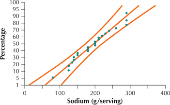
Sodium in Breakfast Cereal. Use the following information for Exercises 78–83. A random sample of 23 breakfast cereals containing sodium had a mean sodium content per serving of 192.39 grams. Assume that the population standard deviation equals 50 grams. We are interested in whether the population mean sodium content per serving is less than 210 grams.

Question 9.184

78. Based on the normal probability plot of the sodium content in the accompanying figure, should we proceed to apply the Z test? Why or why not?

Question 9.185

79. Assuming that the normal probability plot shows acceptable normality, we will test whether the population mean sodium content per serving is less than 210 grams, using level of significance $α = 0.01$ .

State the hypotheses and the rejection rule. Make sure you state the meaning of $μ$ .
Calculate $Z_{data}$ .
Find the $p$ -value. Draw a normal probability curve indicating $Z_{data}$ and the $p$ -value.
State the conclusion and the interpretation.

9.3.79

(a) $H_{0} : μ = 210 vs . H_{a} : μ < 210$ , where $μ$ refers to the population mean sodium content per serving of breakfast cereal. We will reject $H_{0}$ if the $p -value \leq α = 0.01$ . (b) $Z_{data} = - 1.69$ . (c) $p -value = 0.0455$

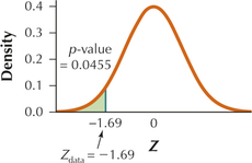
(d) The $p -value = 0.0455$ is not $\leq 0.01$ . Therefore we do not reject $H_{0}$ .

Question 9.186

80. For the $p$ -value in Exercise 79, assess the strength of evidence against the null hypothesis.

Question 9.187

81. Use the equivalence between two-tailed hypothesis tests and confidence intervals to perform a set of hypothesis tests, as follows.

Construct a 95% Z confidence interval for the population mean sodium content. (Hint: See Section 8.1.)
Use the confidence interval to test, at level of significance $α = 0.05$ , whether the population mean sodium content differs from the following amounts:
1. 200
2. 215
3. 170
4. 160

9.3.81

(a) (171.96, 212.82)

(b)

	Value of $μ_{o}$	Form of hypothesis test, with $α = 0.05$	Where $μ_{o}$ lies in relation to 95% confidence interval	Conclusion of hypothesis test
(i)	200	$H_{0} : μ = 200 vs . H_{a} : μ \neq 200$	Inside	Do not reject $H_{0}$
(ii)	215	$H_{0} : μ = 215 vs . H_{a} : μ \neq 215$	Outside	Reject $H_{0}$
(iii)	170	$H_{0} : μ = 170 vs . H_{a} : μ \neq 170$	Outside	Reject $H_{0}$
(iv)	160	$H_{0} : μ = 160 vs . H_{a} : μ \neq 160$	Outside	Reject $H_{0}$

Question 9.188

82. Refer to the hypothesis test in Exercise 79. What if the population standard deviation of 50 grams had been a typo, and the actual population standard deviation was smaller? How would this have affected the following?

The standard deviation of the sampling distribution
$Z_{data}$
$p$ -value
The conclusion

Question 9.189

83. Refer to the hypothesis test in Exercise 79. What if our level of significance $α$ equaled 0.05 instead of 0.01?

Perform the appropriate hypothesis test using the $p$ -value method, but this time using level of significance $α = 0.05$ .
Note that your conclusion differs from that obtained using level of significance $α = 0.01$ . Have the data changed? Why did your conclusion change?
Suggest two alternatives for addressing the contradiction between Exercise 79 and Exercise 83(a).

9.3.83

(a) $H_{0} : μ = 210 vs . H_{a} : μ < 210$ . Reject $H_{0}$ if $p -value \leq 0.05$ . $Z_{data} = - 1.69$ . $p -value = 0.0455$ . Since $p -value = 0.0455$ is $\leq α = 0.05$ , reject $H_{0}$ . There is evidence that the population mean sodium content per serving of breakfast cereal is less than 210 grams. (b) The data have not changed; $α$ was increased to a value greater than the $p -value$ . (c) Report the $p -value$ and assess the strength of the evidence against the null hypothesis; obtain more data.

WORKING WITH LARGE DATA SETS

Texas Towns. Work with the Texas data set for Exercises 84–86.

Question 9.190

texas

84. How many observations are in the data set? How many variables?

Question 9.191

texas

85. Use technology to explore the variable tot_occ, which lists the total occupied housing units for each county in Texas. Generate numerical summary statistics and graphs for the total occupied housing units. What is the sample mean? The sample standard deviation? Comment on the symmetry or skewness of the data set.

9.3.85

$\bar{x} = 23, 901$ , $s = 88, 421$ . The distribution is right-skewed.

Question 9.192

texas

86. Suppose we are using the data in this data set as a sample of the total occupied housing units of all the counties in the southwestern United States, and let $σ = 88, 400$ . Use technology to test, at level of significance $α = 0.05$ , whether the population mean total occupied housing units for these counties differs from 40,000.

WORKING WITH LARGE DATA SETS

Chapter 9 Case Study: Clothing Store Sales. Open the Chapter 9 Case Study data set, Clothing Store. Here, we will perform a hypothesis test for the population mean number of items purchased per customer. We will then see whether this hypothesis test made the correct decision. Use technology to do the following exercises.

Question 9.193

clothingstore

87. Obtain a random sample of size 100 from the data set.

9.3.87

Answers will vary.

Question 9.194

88. The assistant manager wants to determine whether the mean number of items customers are buying is less than 20. Using your sample, perform the appropriate hypothesis test, using level of significance $α = 0.05$ . Assume $σ = 25$ .

Question 9.195

89. Using the same sample, test whether the population mean number of items purchased per customer is less than 18, using level of significance $α = 0.05$ . Assume $σ = 25$ .

9.3.89

$H_{0} : μ = 18 vs . H_{a} : μ < 18$ . We will reject $H_{0}$ if the $p -value \leq α = 0.05.$

Answers will vary for the rest of the problem.

Question 9.196

90. Find the actual value of the population mean number of items purchased per customer.

Did your hypothesis test in Exercise 89 make the right decision? Explain.
Discuss the decision your hypothesis test in Exercise 89 made, using the concept of “beyond a reasonable doubt.”