1.1 Limits of Functions Using Numerical and Graphical TechniquesPrinted Page 69
69
OBJECTIVES
When you finish this section, you should be able to:
Calculus can be used to solve certain fundamental questions in geometry. Two of these questions are:
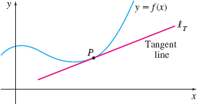
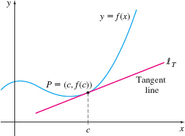
- Given a function \(f\) and a point \(P\) on its graph, what is the slope of the line tangent to the graph of \(f\) at \(P\)? See Figure 1.
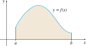
- Given a nonnegative function \(f\) whose domain is the closed interval \([a,b]\), what is the area enclosed by the graph of \(f\), the \(x\)-axis, and the vertical lines \(x=a\) and \(x=b\)? See Figure 2.


These questions, traditionally called the tangent problem and the area problem, were solved by Gottfried Wilhelm von Leibniz and Sir Isaac Newton during the late seventeenth and early eighteenth centuries. The solutions to the two seemingly different problems are both based on the idea of a limit. Their solutions not only are related to each other, but are also applicable to many other problems in science and geometry. Here, we begin to discuss the tangent problem. The discussion of the area problem begins in Chapter 5.
1 Discuss the Slope of a Tangent Line to a GraphPrinted Page 69
Notice that the line \(\ell_{T}\) in Figure 1 just touches the graph of \(f\) at the point \(P\). This unique line is the tangent line to the graph of \(f\) at \(P\). But how is the tangent line defined?
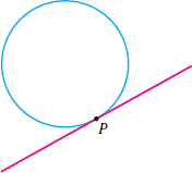
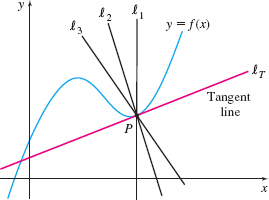
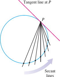
In plane geometry, a tangent line to a circle is defined as a line having exactly one point in common with the circle, as shown in Figure 3. However, this definition does not work for graphs in general. For example, in Figure 4, three lines \(\ell_{1}\), \(\ell_{2}\), and \(\ell_{3}\) contain the point \(P\) and have exactly one point in common with the graph of \(f\), but they do not meet the requirement of just touching the graph at \(P\). On the other hand, the line \(\ell_{T}\) just touches the graph of \(f\) at \(P\), but it intersects the graph at other points. It is the slope of the tangent line \(\ell_{T}\) that distinguishes it from all other lines containing \(P\).
NEED TO REVIEW?
The slope of a line is discussed in Appendix A.3, p. A-18.
So before defining a tangent line, we investigate its slope, which we denote by \(m_{\tan}\). We begin with the graph of a function \(f\), a point \(P\) on its graph, and the tangent line \(\ell_{T}\) to \(f\) at \(P\), as shown in Figure 5.
The tangent line \(\ell_{T}\) to the graph of \(f\) at \(P\) must contain the point \(P\). We denote the coordinates of \(P\) by \(( c,f(c) )\). Since finding slope requires two points, and we have only one point on the tangent line \(\ell_{T}\), we need another way to find the slope of \(\ell_{T}\).
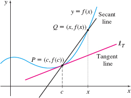
Suppose we choose any point \(Q=({x,f(x)})\), other than \(P\), on the graph of \(f\), as shown in Figure 6. (\(Q\) can be to the left or to the right of \(P\); we chose \(Q\) to be to the right of \(P\).) The line containing the points \(P=(c, f(c))\) and \(Q= (x,f(x))\) is called a secant line of the graph of \(f\). The slope \(m_{\text{sec}}\) of this secant line is \[\bbox[5px, border:1px solid black, #F9F7ED]{\bbox[#FAF8ED,5pt]m_{\sec }=\dfrac{f( x) -f( c) }{x-c}}\tag{1} \]
70
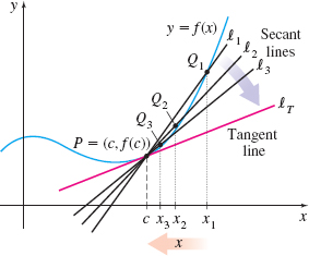
Figure 7 shows three different points \(Q_{1}\), \(Q_{2}\), and \(Q_{3}\) on the graph of \(f\) that are successively closer to point \(P\), and three associated secant lines \(\ell_{1}\), \(\ell_{2}\), and \(\ell_{3}\). The closer the point \(Q\) is to the point \(P\), the closer the secant line is to the tangent line \(\ell_{T}\). The line \(\ell_{T}\), the limiting position of these secant lines, is the tangent line to the graph of \(f\) at \(P\).
As Figure 8 illustrates, this new idea of a tangent line is consistent with the traditional definition of a tangent line to a circle.
If the limiting position of the secant lines is the tangent line, then the limit of the slopes of the secant lines should equal the slope of the tangent line. Notice in Figure 7 that as the point \(Q\) moves closer to the point \(P\), the numbers \(x\) get closer to \(c\). So, equation (1) suggests that \[ \begin{eqnarray*} m_{\tan }&=& [\hbox{Slope of the tangent line to }f\hbox{ at }P] \\[4pt] &=& \left[ \hbox{Limit of }{\dfrac{f(x) -f(c) }{x-c} }\hbox{ as }x\hbox{ gets closer to }c\right] \end{eqnarray*} \]
In symbols, we write \[ \begin{equation*} m_{\tan }=\lim\limits_{x\rightarrow c}\frac{f( x) -f( c) }{x-c} \end{equation*} \]
The notation \(\lim\limits_{x\rightarrow c}\) is read, “the limit as \(x\) approaches \(c\).”
The tangent line to the graph of a function \(f\) at a point \(P=(c,f(c))\) is the line containing the point \(P\) whose slope is \[\bbox[5px, border:1px solid black, #F9F7ED]{m_{\tan}=\lim\limits_{x\rightarrow c}\dfrac{f(x)-f(c)}{x-c}} \]
provided the limit exists.
NOTE
We discuss what it means for a limit to exist shortly.
We have begun to answer the tangent problem by introducing the idea of a limit. Now we describe the idea of a limit in more detail.
The Idea of a Limit
NEED TO REVIEW?
If \(a\lt b\), the open interval \((a, b)\) consists of all numbers \(x\) for which \(a\lt x\lt b\). Interval notation is discussed in Appendix A.1, p. A-5.
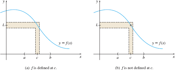
We begin by asking a question: What does it mean for a function \(f\) to have a limit \(L\) as \(x\) approaches some fixed number \(c\)? To answer the question, we need to be more precise about \(f\), \(L\), and \(c\). The function \(f\) must be defined everywhere in an open interval containing the number \(c\), except possibly at \(c\), and \(L\) is a number. Using these restrictions, we introduce the notation \[\bbox[5px, border:1px solid black, #F9F7ED]{\lim\limits_{x\rightarrow c}f(x)=L} \]
71
which is read, “the limit as \(x\) approaches \(c\) of \(f(x)\) is equal to the number \(L\).” The notation \(\lim\limits_{x\rightarrow c}f(x)=L\) can be described as
The value \(f(x)\) can be made as close as we please to \(L\), for \(x\) sufficiently close to \(c\), but not equal to \(c\).
See Figure 9.
2 Investigate a Limit Using a Table of NumbersPrinted Page 71
EXAMPLE 1Investigating a Limit Using a Table of Numbers
Investigate \(\lim\limits_{x\rightarrow 2}( 2x+5)\) using a table of numbers.
Solution We create Table 1 by evaluating \(f(x) =2x+5\) at values of \(x\) near 2, choosing numbers \(x\) slightly less than 2 and numbers \(x\) slightly greater than 2.
| \(\underrightarrow{\hbox{numbers \(x\) slightly less than 2}}\) | \(\underleftarrow{\hbox{numbers \(x\) slightly greater than 2}}\) | ||||||||||
|---|---|---|---|---|---|---|---|---|---|---|---|
| \(x\) | 1.99 | 1.999 | 1.9999 | 1.99999 | \(\rightarrow\) | 2 | \(\leftarrow\) | 2.00001 | 2.0001 | 2.001 | 2.01 |
| \(f(x) =2x+5\) | 8.98 | 8.998 | 8.9998 | 8.99998 | \(f(x)\) approaches 9 | 9.00002 | 9.0002 | 9.002 | 9.02 | ||
Table 1 suggests that the value of \(f(x)=2x+5\) can be made “as close as we please” to 9 by choosing \(x\) “sufficiently close” to 2. This suggests that \(\lim\limits_{x\rightarrow 2}( 2x+5) =9\).
NOW WORK
In creating Table 1, first we used numbers \(x\) close to 2 but less than 2 , and then we used numbers \(x\) close to 2 but greater than 2. When \(x\lt 2\) , we say, “\(x\) is approaching 2 from the left,” and the number 9 is called the left-hand limit. When \(x\gt 2\), we say, “\(x\) is approaching 2 from the right,” and the number 9 is called the right-hand limit. Together, these are called the one-sided limits of \(f\) as \(x\) approaches 2.
One-sided limits are symbolized as follows. The left-hand limit, written \[\bbox[5px, border:1px solid black, #F9F7ED]{ \lim\limits_{^{{}}x\rightarrow c^{-}}f(x)=L_{{\rm left}} } \]
is read, “The limit as \(x\) approaches \(c\) from the left of \(f(x)\), equals \(L_{\text{left}}\).” It means that the value of \(f\) can be made as close as we please to the number \(L_{\text{left}}\) by choosing \(x\lt c\) and sufficiently close to \(c\).
Similarly, the right-hand limit, written \[\bbox[5px, border:1px solid black, #F9F7ED]{ \lim\limits_{x\rightarrow c^{+}}f(x)=L_{\text{right}} } \]
72
and is read, “The limit as \(x\) approaches \(c\) from the right of \(f(x)\), equals \(L_{\text{right}}\).” It means that the value of \(f\) can be made as close as we please to the number \(L_{\text{right}}\) by choosing \(x>c\) and sufficiently close to \(c\).
EXAMPLE 2Investigating a Limit Using a Table of Numbers
Investigate \(\lim\limits_{x\rightarrow 0}\dfrac{e^{x}-1}{x}\) using a table of numbers.
Solution The domain of \(f(x)=\dfrac{e^{x}-1}{x}\) is \(\{x| x\neq 0 \}\). So, \(f\) is defined everywhere in an open interval containing the number 0, except for 0.
We create Table 2, investigating the left-hand limit \(\lim\limits_{x\rightarrow 0^{-}}\dfrac{e^{x}-1}{x}\) and the right-hand limit \(\lim\limits_{x\rightarrow 0^{+}}\dfrac{e^{x}-1}{x}\). First, we evaluate \(f\) at numbers less than 0, but close to zero, and then at numbers greater than 0, but close to zero.
| \(\underrightarrow{x~\hbox{approaches 0 from the left}}\) | \(\underleftarrow{x~\hbox{approaches 0 from the right}}\) | ||||||||||
|---|---|---|---|---|---|---|---|---|---|---|---|
| \(x\) | -0.01 | -0.001 | -0.0001 | -0.00001 | \(\rightarrow\) | 0 | \(\leftarrow\) | 0.00001 | 0.0001 | 0.001 | 0.01 |
| \(f(x) =\dfrac{e^{x}-1}{x}\) | 0.995 | 0.9995 | 0.99995 | 0.999995 | \(f(x)\) approaches 1 | 1.000005 | 1.00005 | 1.0005 | 1.005 | ||
Table 2 suggests that \(\lim\limits_{x\rightarrow 0^{-}}\dfrac{e^{x}-1}{x}=1\) and \(\lim\limits_{x\rightarrow 0^{+}}\dfrac{e^{x}-1}{x}=1\). This suggests \(\lim\limits_{x\rightarrow 0}\dfrac{e^{x}-1}{x}=1\).
NOW WORK
NOTE
\({f(x)=}\dfrac{\sin {x}}{{x}}\) is an even function, so the bottom row of Table 3 is symmetric about \(x=0\).
EXAMPLE 3Investigating a Limit Using a Table of Numbers
Investigate \(\lim\limits_{x\rightarrow 0}\dfrac{\sin x}{x}\) using a table of numbers.
Solution The domain of the function \(f(x)=\dfrac{\sin x}{x}\) is \(\{x~|~x\neq 0\}\). So, \(f\) is defined everywhere in an open interval containing 0, except for 0.
We create Table 3, by investigating one-sided limits of \(\dfrac{\sin x}{x}\) as \(x\) approaches 0, choosing numbers (in radians) slightly less than 0 and numbers slightly greater than 0.
| \(\underrightarrow{x~\hbox{approaches 0 from the left}}\) | \(\underleftarrow{x~\hbox{approaches 0 from the right}}\) | ||||||||||
|---|---|---|---|---|---|---|---|---|---|---|---|
| \(x\) (in radians) | -0.02 | -0.01 | 0.005 | \(\rightarrow\) | 0 | \(\leftarrow\) | 0.005 | 0.01 | 0.02 | ||
| \(f(x) =\dfrac{\sin x}{x}\) | 0.99993 | 0.99998 | 0.999996 | \(f(x)\) approaches 1 | 0.999996 | 0.99998 | 0.99993 | ||||
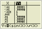
Table 3 suggests that \(\lim\limits_{x\rightarrow 0^{-}}f(x)=1\) and \(\lim\limits_{x\rightarrow 0^{+}}f(x)=1\). This suggests that \(\lim\limits_{x\rightarrow 0}\dfrac{\sin x}{x}=1\).
73
The table used to investigate the limit can be created using technology, as shown in Figure 10.
NOW WORK
3 Investigate a Limit Using a GraphPrinted Page 73
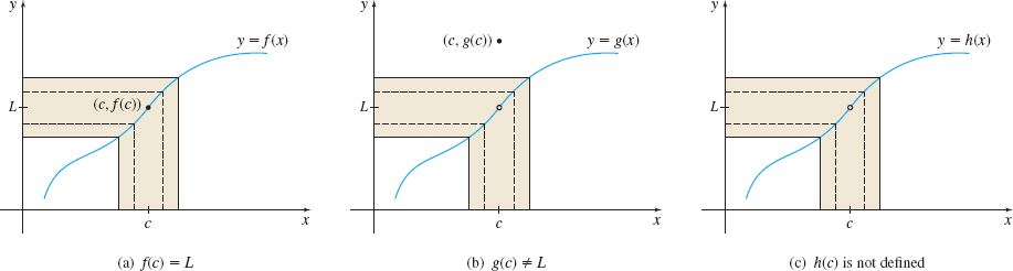
The graph of a function can also help us investigate limits. Figure 11 shows the graphs of three different functions \(f\), \(g\), and \(h\). Observe that in each function, as \(x\) gets closer to c, whether from the left or from the right, the value of the function gets closer to the number L. This is the key idea of a limit.
Notice in Figure 11(b) that the value of \(g\) at \(c\) does not affect the limit. Notice in Figure 11(c) that \(h\) is not defined at \(c\), but the value of \(h\) gets closer to the number \(L\) for \(x\) sufficiently close to \(c\). This suggests that the limit of each function as \(x\) approaches \(c\) is \(L\) even though the values of each function at \(c\) are different.
EXAMPLE 4Investigating a Limit Using a Graph
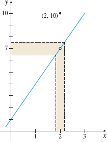
Use a graph to investigate \(\lim\limits_{x\rightarrow 2}f( x)\) if \(f(x)=\left\{ \begin{array}{c@{\qquad}l} 3x+1 & \hbox{if }\quad x\neq 2 \\ 10 & \hbox{if }\quad x=2 \end{array} \right. . \)
NEED TO REVIEW?
Piecewise-defined functions are discussed in Section P.1, p. 7.
Solution The function \(f\) is a piecewise-defined function. Its graph is shown in Figure 12. Observe that as \(x\) approaches 2 from the left, the value of \(f\) is close to 7, and as \(x\) approaches 2 from the right, the value of \(f\) is close to 7. In fact, we can make the value of \(f\) as close as we please to 7 by choosing \(x\) sufficiently close to 2 but not equal to 2. This suggests \(\lim\limits_{x\rightarrow 2}f(x)=7\).
If we use a table of numbers to investigate \(\lim\limits_{x\rightarrow2}f( x)\), the result is the same. See Table 4.
| \(\underrightarrow{x~\hbox{approaches 2 from the left}}\) | \(\underleftarrow{x~\hbox{approaches 2 from the right}}\) | ||||||||||
|---|---|---|---|---|---|---|---|---|---|---|---|
| \(x\) | 1.99 | 1.999 | 1.9999 | 1.99999 | \(\rightarrow\) | 2 | \(\leftarrow\) | 2.00001 | 2.0001 | 2.001 | 2.01 |
| \(f(x)\) | 6.97 | 6.997 | 6.9997 | 6.99997 | \(f(x)\) approaches 7 | 7.00003 | 7.0003 | 7.003 | 7.03 | ||
Figure 12 shows that \(f(2)=10\), but that this value has no impact on the limit as \(x\) approaches 2.
74
We make the following observations:
- The limit \(L\) of a function \(y=f(x)\) as \(x\) approaches a number \(c\) does not depend on the value of \(f\) at \(c\).
- The limit \(L\) of a function \(y=f(x)\) as \(x\) approaches a number \(c\) is unique; that is, a function cannot have more than one limit. (A proof of this property is given in Appendix B.)
- If there is no single number that the value of \(f\) approaches as \(x\) gets close to \(c\), we say that f has no limit as \(x\) approaches, or more simply, that the limit of \(f\) does not exist at \(c\).
Example 5 and Example 6 that follow illustrate situations in which a limit doesn’t exist.

EXAMPLE 5Investigating a Limit Using a Graph
Use a graph to investigate \(\lim\limits_{x\rightarrow 0}f(x)\) if \(f( x) =\left\{ \begin{array}{l@{\qquad}l} x & \hbox{if }\quad x<0 \\ 1 & \hbox{if }\quad x>0 \end{array} \right. .\)
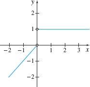
Solution Figure 13 shows the graph of \(f\). We first investigate the one-sided limits. The graph suggests that, as \(x\) approaches 0 from the left, \[ \begin{equation*} \lim_{x\rightarrow 0^{-}}f(x)=0 \end{equation*} \]
and as \(x\) approaches 0 from the right, \[ \begin{equation*} \lim_{x\rightarrow 0^{+}}f(x)=1 \end{equation*} \]
Since there is no single number that the values of \(f\) approach when \(x\) is close to 0, we conclude that \(\lim\limits_{x\rightarrow 0}f(x)\) does not exist.
Table 5 uses a numerical approach to support the conclusion that \(\lim\limits_{x\rightarrow 0}f(x)\) does not exist.
| \(\underrightarrow{x~\hbox{approaches 0 from the left}}\) | \(\underleftarrow{x~\hbox{approaches 0 from the right}}\) | ||||||||
|---|---|---|---|---|---|---|---|---|---|
| \(x\) | –0.01 | –0.001 | –0.0001 | \(\rightarrow\) | 0 | \(\leftarrow\) | 0.0001 | 0.001 | 0.01 |
| \(f(x)\) | –0.01 | –0.001 | –0.0001 | no single number | 1 | 1 | 1 | ||
Example 4 and Example 5 lead to the following result.
THEOREM
The limit \(L\) of a function \(y=f(x)\) as \(x\) approaches a number \(c\) exists if and only if both one-sided limits exist at \(c\) and both one-sided limits are equal. That is, \[ \begin{equation*} \ \ \ \ \ \lim\limits_{x\rightarrow c}f( x) =L\quad \hbox{ if and only if }\quad \lim\limits_{^{{}}x\rightarrow c^{-}}f(x) =\lim\limits_{x\rightarrow c^{+}}f( x) =L \ \ \ \ \ \end{equation*} \]
NOW WORK
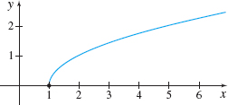
A one-sided limit is used to describe the behavior of functions such as \(f(x)=\sqrt{x-1}\) near \(x=1\). Since the domain of \(f\) is \(\{x|x\geq 1\}\), the left-hand limit, \(\lim\limits_{x\rightarrow 1^{-}}\sqrt{x-1}\) makes no sense. But \(\lim\limits_{x\rightarrow 1^{+}}\sqrt{x-1}=0\) suggests how \(f\) behaves near and to the right of 1. See Figure 14 and Table 6. They suggest \(\lim\limits_{x\rightarrow 1^{+}} f(x)=0\).
| \(\underrightarrow{x~\hbox{approaches 1 from the right}}\) | ||||||
|---|---|---|---|---|---|---|
| \(x\) | 1.009 | 1.0009 | 1.00009 | 1.000009 | 1.0000009 | \(\rightarrow\) 1 |
| \(f(x) =\sqrt{x-1}\) | 0.0949 | 0.03 | 0.00949 | 0.003 | 0.000949 | \(f(x)\) approaches 0 |
75
Using numeric tables and/or graphs gives us an idea of what a limit might be. That is, these methods suggest a limit, but there are dangers in using these methods, as the following example illustrates.
EXAMPLE 6Investigating a Limit
Investigate \(\lim\limits_{x\rightarrow 0}\sin \dfrac{\pi}{x^{2}}\).
Solution The domain of the function \(f(x)=\sin \dfrac{\pi }{x^{2}}\) is \(\{x|x\neq 0\}\). Suppose we let \(x\) approach zero in the following way:
| \(\underrightarrow{x~\hbox{approaches 0 from the left}}\) | \(\underleftarrow{x~\hbox{approaches 0 from the right}}\) | ||||||||||
|---|---|---|---|---|---|---|---|---|---|---|---|
| \(x\) | \(-\dfrac{1}{10}\) | \(-\dfrac{1}{100}\) | \(-\dfrac{1}{1000}\) | \(-\dfrac{1}{10{,}000}\) | \(\rightarrow\) | 0 | \(\leftarrow\) | \(\dfrac{1}{10,000}\) | \(\dfrac{1}{1000}\) | \(\dfrac{1}{100}\) | \(\dfrac{1}{10}\) |
| \(f(x) =\sin \dfrac{\pi }{x^{2}}\) | 0 | 0 | 0 | 0 | \(f(x)\) approaches 0 | 0 | 0 | 0 | 0 | ||
The table suggests that \(\lim\limits_{x\rightarrow 0}\sin \dfrac{\pi }{x^{2}}=0\). Now suppose we let \(x\) approach zero as follows:
| \(\underrightarrow{x~\hbox{approaches 0 from the left}}\) | \(\underleftarrow{x~\hbox{approaches 0 from the right}}\) | ||||||||||||
|---|---|---|---|---|---|---|---|---|---|---|---|---|---|
| \(x\) | \(-\dfrac{2}{3}\) | \(-\dfrac{2}{5}\) | \(-\dfrac{2}{7}\) | \(-\dfrac{2}{9}\) | \(-\dfrac{2}{11}\) | \(\rightarrow\) | 0 | \(\leftarrow\) | \(\dfrac{2}{11}\) | \(\dfrac{2}{9}\) | \(\dfrac{2}{7}\) | \(\dfrac{2}{5}\) | \(\dfrac{2}{3}\) |
| \(f(x) =\sin\dfrac{\pi}{x^{2}}\) | 0.707 | 0.707 | 0.707 | 0.707 | 0.707 | \(f(x)\) approaches 0.707 | 0.707 | 0.707 | 0.707 | 0.707 | 0.707 | ||
This table suggests that \(\lim\limits_{x\rightarrow 0}\sin \dfrac{\pi }{x^{2}}=\dfrac{\sqrt{2}}{2}\approx 0.707\).
In fact, by carefully selecting \(x\), we can make \(f\) appear to approach any number in the interval \([-1, 1]\).
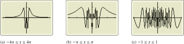
Now look at the graphs of \(f(x) =\sin \dfrac{\pi}{x^{2}}\) shown in Figure 15. In Figure 15(a), the choice of \(\lim\limits_{x\rightarrow0}\sin \dfrac{\pi }{x^{2}}=0\) seems reasonable. But in Figure 15(b), it appears that \(\lim\limits_{x\rightarrow 0}\sin \dfrac{\pi }{x^{2}}=-\dfrac{1 }{2}\). Figure 15(c) illustrates that the graph of \(f\) oscillates rapidly as \(x\) approaches 0. This suggests that the value of \(f\) does not approach a single number, and that \(\lim\limits_{x\rightarrow 0}\sin \dfrac{\pi }{x^{2}}\) does not exist.
NOW WORK
So, how do we find a limit with certainty? The answer lies in giving a very precise definition of limit. The next example helps explain the definition.
76
EXAMPLE 7Analyzing a Limit
In Example 1, we claimed that \(\lim\limits_{x\rightarrow 2}(2x+5) =9\).
- (a) How close must \(x\) be to 2, so that \(f(x) =2x+5\) is within 0.1 of 9?
- (b) How close must \(x\) be to 2, so that \(f(x) =2x+5\) is within 0.05 of 9?
RECALL
On the number line, the distance between two points with coordinates \({a}\) and \(b\) is \(\vert{a-b}\vert\).
Solution (a) The function \(f(x)=2x+5\) is within 0.1 of 9, if the distance between \(f(x)\) and 9 is less than 0.1 unit. That is, if \(\vert f(x)-9\vert\leq 0.1\). \[ \begin{eqnarray*} \vert (2x+5) -9\vert &\leq &0.1 \\ \vert 2x-4\vert &\leq &0.1 \\ \vert 2( x-2) \vert &\leq &0.1 \\ \vert x-2\vert &\leq &\dfrac{0.1}{2}=0.05 \\ -0.05 &\leq &x-2\leq 0.05 \\ 1.95 &\leq &x\leq 2.05 \end{eqnarray*} \]
NEED TO REVIEW?
Inequalities involving absolute values are discussed in Appendix A.1, p. A-7.
So, if \(1.95\leq x\leq 2.05\), then \(f(x)\) will be within 0.1 of 9.
(b)The function \(f(x)=2x+5\) is within 0.05 of 9 if \(\vert f(x) -9\vert \leq 0.05\). That is, \[ \begin{eqnarray*} \vert ( 2x+5) -9\vert &\leq &0.05 \\ \vert 2x-4\vert &\leq &0.05 \\ \vert x-2\vert &\leq &\dfrac{0.05}{2}=0.025 \end{eqnarray*} \]
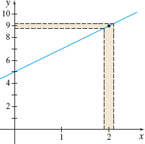
So, if \(1.975\leq x\leq 2.025\), then \(f(x)\) will be within 0.05 of 9.
Notice that the closer we require \(f\) to be to the limit 9, the narrower the interval for \(x\) becomes. See Figure 16.
NOW WORK
The discussion in Example 7 forms the basis of the definition of a limit. We state the definition here, but postpone the details until Section 1.6. It is customary to use the Greek letters \(\epsilon\) (epsilon) and \(\delta\) (delta) in the definition, so we call it the \(\epsilon\)-\(\delta\) definition of a limit.
DEFINITION \(\epsilon\)-\(\delta\) Definition of a Limit
Let \(f\) be a function defined everywhere in an open interval containing \(c\), except possibly at \(c\). Then the limit of the function \(f\) as \(x\) approaches \(c\) is the number \(L\), written \[\bbox[5px, border:1px solid black, #F9F7ED]{\lim\limits_{x\rightarrow c}f(x)=L} \]
if, given any number \(\epsilon \gt 0\), there is a number \(\delta \gt 0\) so that \[\bbox[5px, border:1px solid black, #F9F7ED]{\hbox{whenever }0< \vert x-c \vert <\delta \quad \hbox{ then } \vert f(x)-L \vert <\epsilon} \]
Notice in the definition that \(f\) is defined everywhere in an open interval containing \(c\) except possibly at \(c\). If \(f\) is defined at \(c\) and there is an open interval containing \(c\) that contains no other numbers in the domain of \(f\), then \(\lim\limits_{x\rightarrow c}f(x)\) does not exist.