14.3 Wilcoxon Signed Rank Test for Matched-Pair Data
 This page includes Video Technology Manuals
OBJECTIVES By the end of this section, I will be able to …
- Assess whether or not a data set is symmetric.
- Perform the Wilcoxon signed rank test for matched-pair data from two dependent samples.
- Perform the Wilcoxon signed rank test for a single population median.
The sign test that we learned about in Section 14.2 required only that the sample be randomly selected. However, because the requirements for performing the sign test are so minimal, the efficiency of the sign test may not be as high as the analyst would want it to be.
If the sample data are randomly selected and symmetric, however, the data analyst may apply the more efficient Wilcoxon signed rank test to two of the situations in which the sign test can be applied, namely, to test for a single population median and to test for the population median of the differences for matched-pair data.
1 Assessing the Symmetry of a Data Set
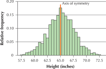
In Section 2.2, we learned that a distribution is symmetric if an axis of symmetry splits the image in half so that one side is the mirror image of the other. The distribution of women's heights in Figure 6 is approximately symmetric (exact symmetry is rarely achieved with real-world data). If the data were randomly selected, it would be appropriate to perform the Wilcoxon signed rank test on the data in Figure 6. On the other hand, the distributions shown in Figures 7 and 8 are not symmetric.
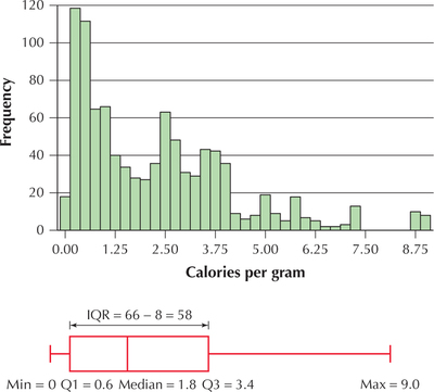
In Section 3.5, we learned that a boxplot is a convenient method for assessing the symmetry of a data set. Figure 7 shows the clearly right-skewed histogram of the number of calories per gram for the food items in the Nutrition data set. Note that the corresponding boxplot has a longer whisker on the right side, and that the median line is somewhat to the left of the center of the box.
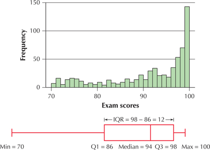
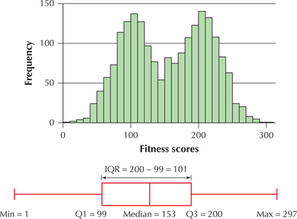
For the left-skewed exam score data in Figure 8, the boxplot has a longer whisker on the left side, and the median line is somewhat to the right of center. Finally, for the symmetric fitness score data in Figure 9, the corresponding boxplot has whiskers of approximately equal length, and the median line is situated approximately in the center of the box.
Boxplot Criterion for Assessing Symmetry
A data set is symmetric when its corresponding boxplot has whiskers of approximately equal length, and the median line is situated approximately in the center of the box.
EXAMPLE 8 Assessing symmetry using the Ti-83/84
In Example 18 in Chapter 9, we examined a random sample of n=20 young women who were admitted with the diagnosis of anorexia nervosa to the Toronto Hospital for Sick Children. Use the TI-83/84 to assess the symmetry of the ages of these women (data on page 526).
Solution
Figure 10 shows the TI-83/84 boxplot of the ages of the young women. The whiskers are of approximately equal length, and the median line is situated approximately in the center of the box. We therefore conclude that the age data are symmetric.
NOW YOU CAN DO
Exercises 11–14.
2 Wilcoxon Signed Rank Test for Matched-Pair Data from two Dependent Samples
In Section 14.2, we performed the sign test to test for both a single population median and for the population median of the difference between two dependent samples. Similarly, in Section 14.3 we apply the Wilcoxon signed rank test for these two situations. We begin with the Wilcoxon signed rank test for matched-pair data from two dependent samples.
In the sign test, the data are converted into plus signs or minus signs. The magnitude of the data values is lost, which contributes to the low efficiency of the sign test. In 1945, Frank Wilcoxon developed the Wilcoxon signed rank test for a single population median, which takes the magnitude of the data into account by ranking the data values.
The Wilcoxon signed rank test is a nonparametric hypothesis test in which the original data are transformed into their ranks. The Wilcoxon signed rank test may be conducted for (a) a single population median or (b) matched-pair data from two dependent samples.
The following example illustrates how to calculate the signed ranks for the Wilcoxon signed rank test.
EXAMPLE 9 Calculating the Wilcoxon signed ranks
The California Community Colleges Chancellor's Office publishes enrollment data for each of its community colleges. Table 7 contains the number of students enrolled in the Spring 2013 and the Spring 2014 semesters at a random sample of six community colleges in California. We are interested in testing whether the median number of enrolled students has declined from 2013 to 2014. That is, we are interested in testing whether the population median of the differences (2014 – 2013) is less than zero.
- Calculate the signed rank for each community college.
- Find the sums of the positive signed ranks and the negative signed ranks.
Solution
Calculate the signed ranks as follows:
- For each data value, find the difference d between the data values for each matched pair. That is, for each community college, we find d = the number of enrolled students in 2014 minus the number of enrolled students in 2013. Omit observations where d=0. These differences are shown in Column 4 of Table 7.
- Find the absolute values of the differences. The absolute values of the differences |d| are shown in Column 5 of Table 7.
- Rank the absolute values of the differences from smallest to largest. If two or more data values are tied with the same rank, assign to each the mean value of their ranks had they not been tied. (There are no ties in this data set. See Example 11 to see how ties are handled.) The ranks of the absolute differences |d| are shown in Column 6 of Table 7.
- Attach to each rank the sign of its corresponding value of d. This is its signed rank. For example, the rank of |d| for Los Angeles Community College is 3, but the sign of d(−392) for Los Angeles is negative (–). We attach this negative sign to the rank to give us Los Angeles's signed rank of −3. Replace each original data value with its corresponding signed rank. The signed ranks are shown in the last column of Table 7.Table 14.26: Table 7 Students enrolled at California community colleges
Community
collegeEnrollment
Spring 2013Enrollment
Spring 2014Difference d
(2014 – 2013)|d| Rank of |d|
Signed
rankLos Angeles CC 148,754 148,362 –392 392 3 –3 Santa Monica CC 31,719 31,437 –282 282 2 –2 El Camino CC 22,657 22,791 134 134 1 1 North Orange CC 51,780 53,993 2,213 2,213 5 5 Foothill CC 34,415 33,574 –841 841 4 –4 Los Rios CC 75,230 71,911 –3,319 3,319 6 –6
The sum of the positive sign ranks is
1+5=6
The sum of the negative signed ranks is
−3−2−4−6=−15
The procedure for the Wilcoxon signed rank test for matched-pair data is summarized as follows.
Wilcoxon Signed Rank Test for Matched-Pair Data
The requirements are that the sample data be randomly selected and that the distribution of the differences be symmetric. It is not required that the population be normally distributed.
Step 1 State the hypotheses.
Choose one of the forms in Table 8.
Table 14.27: Table 8 Hypotheses for the Wilcoxon signed rank test for matched-pair dataNull hypothesis Alternative hypothesis Type of test H0:Md=0 Ha:Md>0 Right-tailed test H0:Md=0 Ha:Md<0 Left-tailed test H0:Md=0 Ha:Md≠0 Two-tailed test - Step 2 Find the critical value and state the rejection rule.
- Small-Sample Case (n≤30): Use Appendix Table J. Choose the column with the appropriate level of significance (α) and the applicable one-tailed or two-tailed test. Then select the row with the appropriate sample size n, where n is the number of data values for which d does not equal zero. The number in that row and column is your critical value Tcrit. The rejection rule is to reject H0 if Tdata≤Tcrit
- Large-Sample Case (n>30): Use Appendix Table C, the standard normal table. The Z critical value for this sign test is always found in the left tail of the standard normal distribution, so that Zcrit is always less than 0. For a left-tailed test or a right-tailed test, the critical value Zcrit is the value of Z with area α to the left of it. For a two-tailed test, the critical value Zcrit is the value of Z with area α/2 to the left of it. Table 4 in Chapter 9 (page 500) contains values of Zcrit for some common values of α. The rejection rule is to reject H0 if Zdata≤Zcrit
Step 3 Find the value of the test statistic.
First find the signed ranks using the following steps:
- For each data value, find the difference d between each data value and the hypothesized median M0. Omit data values for which d=0.
- Find the absolute values of the differences.
- Rank the absolute values of the differences from smallest to largest. If two or more data values have the same rank, assign to each the mean value of their ranks had they not been tied.
- Attach to each rank the sign of its corresponding value of d. This is its signed rank. Replace each original data value with its corresponding signed rank.
Page 14-22- Small-Sample Case (n≤30): Use Table 9 to find Tdata, where T+ is the sum of the positive signed ranks, and |T−| is the absolute value of the sum of the negative signed ranks.Table 14.28: Table 9 Finding Tdata
Type of test Test statistic Tdata Right-tailed test Tdata= |T−| Left-tailed test Tdata=T+ Two-tailed test Tdata=T+ or |T−|, whichever is smaller - Large-Sample Case (n>30): Use Table 9 to find Tdata, and then calculate the test statistic Zdata:
Zdata=Tdata−n(n+1)4√n(n+1)(2n+1)24
- Step 4 State the conclusion and the interpretation. Compare the test statistic with the critical value, using the rejection rule.
We illustrate the Wilcoxon signed rank test for the population median of the differences using the following example.
EXAMPLE 10 Wilcoxon signed rank test for matched-pair data
Use the data from Example 9 to test whether the population median number of enrolled students M has decreased from 2013 to 2014, using level of significance α=0.05.
Solution
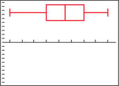
Figure 11 is a TI-83/84 boxplot of the differences (2014 – 2013). The whiskers are approximately the same length, indicating symmetry. Thus, we have a random sample of data exhibiting acceptable symmetry, and so our conditions are met.
Step 1 State the hypotheses. We have a left-tailed test:
H0:Md=0versusHα:Md<0
where M represents the population median of the differences in number of enrolled students at California community colleges from 2013 to 2014.
- Step 2 Find the critical value and state the rejection rule. The sample size is the number of data values for which the difference does not equal zero. Because none of the differences equals zero, our sample size is n=6. Because n≤30, we use the small-sample case. To find the critical value, we use Appendix Table J. We have a one-tailed test, with level of significance α=0.05 and n=6, which gives us Tcrit=2, as shown in Figure 12. The rejection rule is to reject H0 if Tdata≤2.
Step 3 Find the value of the test statistic. The signed ranks are given in Table 7. We have a left-tailed test, so from Table 9, we have
Tdata=T+=the sum of the positive signed ranks=1+5=6
Page 14-23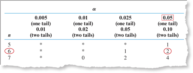 FIGURE 12 Finding the critical value Tcrit.
- Step 4 State the conclusion and the interpretation. Because Tdata=6 is not ≤2, we do not reject H0. The evidence is insufficient to conclude that the population median number of students enrolled at California community colleges has decreased from 2013 to 2014.
NOW YOU CAN DO
Exercises 15–18.
3 Wilcoxon Signed Rank Test for a Single Population Median
We can use the same methods for the Wilcoxon signed rank test for a single population median that we used for the Wilcoxon signed rank test for matched-pair data. However, only one sample is involved, so no subtraction is necessary to find the differences. The hypotheses for the Wilcoxon signed rank test for a single population median are the same as those for the sign test for matched-pair data, given in Table 10.
| Null hypothesis | Alternative hypothesis | Type of test |
|---|---|---|
| H0:M=M0 | Ha:M>M0 | Right-tailed test |
| H0:M=M0 | Ha:M<M0 | Left-tailed test |
| H0:M=M0 | Ha:M≠M0 | Two-tailed test |
We illustrate the small-sample case of the Wilcoxon signed rank test for a single population median using the following example.
EXAMPLE 11 Wilcoxon signed rank test for a single population median: small-sample case
The Web site www.missingkids.com provides a searchable database of missing children. The ages of the following six children were obtained from this database.
| Child | Adam | Juan | Benjamin | Samantha | Kayleen | Aiko |
| Age | 4 | 9 | 5 | 7 | 6 | 3 |
Test, using level of significance α=0.10, whether the population median age of the missing children equals 6 years old.
Solution
Step 1 State the hypotheses. We have a two-tailed test:
H0:M=6versusHα:M≠6
where M represents the population median age of the missing children. Thus, the hypothesized value for the median is M0=6.
- Step 2 Find the critical value and state the rejection rule. To find the critical value, we use Appendix Table J, excerpted here in Figure 13. We have a two-tailed test, with level of significance α=0.10 and n=5, which gives us Tcrit=1. The rejection rule is to reject H0 if Tdata≤1.
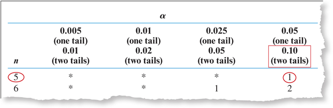 FIGURE 13 Using Appendix Table J to find the critical value Tcrit.
 - Step 3 Find the value of the test statistic. The calculations to find the signed ranks are shown in Table 11.Table 14.31: Table 11 Finding the signed ranks for the child age data
Child Age Age−M0=d |d| Rank of |d| Signed rank Adam 4 4−6=−2 2 3 −3 Juan 9 9−6=3 3 4.5 4.5 Benjamin 5 5−6=−1 1 1.5 −1.5 Samantha 7 7−6=1 1 1.5 1.5 Kayleen 6 6−6=0 — — — Aiko 3 3−6=−3 3 4.5 −4.5 - Find d=age−M0=age−6 for each child. Note that the value of d for Kayleen is zero, so we omit Kayleen's age from further calculations.
- The absolute values of the differences |d| are shown in the fourth column of Table 11.
- We rank the absolute differences. Notice that the absolute values for Benjamin and Samantha are |d|=1. Had they not been tied, their ranks would have been 1 and 2. The mean of 1 and 2 is (1+2)/2=1.5. Thus, each child's age is assigned the rank of 1.5. There is also a tie between Juan and Aiko, with |d|=3. Had they not been tied, their ranks would have been 4 and 5, so each child's age is assigned the mean rank of 4.5. The ranks of the absolute differences |d| are shown in the fifth column of Table 11.
- Attach to each rank the sign of its corresponding value of d. This is its signed rank. For example, the rank of |d| for Adam is 3, but the sign of d=−2 for Adam is negative (–). We attach this negative sign to the rank for Adam to give us Adam's signed rank of –3. Replace each original data value with its corresponding signed rank, shown in the last column of Table 11.
Page 14-25Next, we need to sum the positive ranks and the negative ranks. There are two positive signed ranks: Juan's 4.5 and Samantha's 1.5. Thus, T+=4.5+1.5=6. There are three negative signed ranks, which we add to get T−:−3+(−1.5)+(−4.5)=−9. Taking the absolute value gives us |T−|=|−9|=9. Table 9 tells us that Tdata=the smaller ofT+ and|T−| Thus, Tdata=6.
- Step 4 State the conclusion and the interpretation. The rejection rule is to reject H0 if Tdata≤1. Because Tdata=6 is not ≤1, we do not reject H0. There is insufficient evidence that the population median age of missing children differs from 6 years old.
NOW YOU CAN DO
Exercises 19–22.
EXAMPLE 12 Large-sample Wilcoxon signed rank test for a population median using technology
Test using level of significance α=0.10 whether the population median age of missing children differs from 6 years old, using the random sample of 50 missing children shown here:
| Child | Age | Child | Age | Child | Age | Child | Age |
|---|---|---|---|---|---|---|---|
| Amir | 5 | Carlos | 7 | Octavio | 8 | Christian | 8 |
| Yamile | 5 | Ulisses | 6 | Keoni | 6 | Mario | 8 |
| Kevin | 5 | Alexander | 7 | Lance | 5 | Reya | 5 |
| Hilary | 8 | Adam | 4 | Mason | 5 | Elias | 1 |
| Zitlalit | 7 | Sultan | 6 | Joaquin | 6 | Maurice | 4 |
| Aleida | 8 | Abril | 6 | Adriana | 6 | Samantha | 7 |
| Alexia | 2 | Ramon | 6 | Christopher | 3 | Michael | 9 |
| Juan | 9 | Amari | 4 | Johan | 6 | Carlos | 2 |
| Kevin | 2 | Joliet | 1 | Kassandra | 4 | Lukas | 4 |
| Hazel | 5 | Christopher | 4 | Hiroki | 6 | Kayla | 4 |
| Melissa | 1 | Jonathan | 8 | Kimberly | 5 | Aiko | 3 |
| Kayleen | 6 | Emil | 7 | Diondre | 4 | Lorenzo | 9 |
| Mirynda | 7 | Benjamin | 5 |
Solution
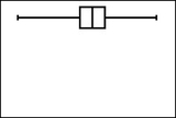
The boxplot of the age data is shown here.
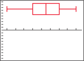
The conditions are met because we have a random sample and the distribution of ages is symmetric.
Step 1 State the hypotheses.
H0:M=6versusHα:M≠6
where M represents the population median age of the missing children.
- Step 2 Find the critical value and state the rejection rule. There are 50 children. Ten of these children are 6 years old, so that d=6−6=0. These 10 children are therefore omitted from this hypothesis test. This leaves us with 40 children, which is greater than 30, so we use the large-sample case. From Table 4 in Chapter 9 (page 500), the two-tailed test with level of significance α=0.10 gives us Zcrit=−1.645. We will reject H0 if Zdata≤−1.645.
Step 3 Find the value of the test statistic. We use the instructions provided in the Step-by-Step Technology Guide at the end of this section. Figure 14 shows the Minitab results, and Figure 15 shows the SPSS results, from the Wilcoxon signed rank test for the population median. Note that the original sample size (“N”) is 50, but that “N for Test” is n=40, because 10 data values have been omitted. The “Wilcoxon Statistic” is the value of Tdata=279, which represents the smaller of T+=279 and |T−|=|−541|=541. We use this value to find the test statistic:
Page 14-26Zdata=Tdata−n(n+1)4√n(n+1)(2n+1)24=279−40(41)4√40(41)(81)24≈−1.7608
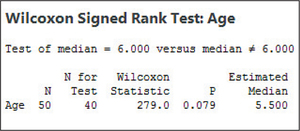 FIGURE 14 Minitab output for the Wilcoxon signed rank test for a population median.
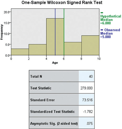 FIGURE 15 SPSS output for the Wilcoxon signed rank test for a population median.
- Step 4 State the conclusion and the interpretation. Because Zdata≈−1.7608≤−1.645, we reject H0. There is evidence that the population median age of the missing children differs from 6 years old. Acquiring more data has changed our conclusion.