11.4 Motion Along a CurvePrinted Page 785
785
OBJECTIVES
When you finish this section, you should be able to:
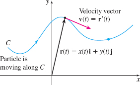
An important physical application of vector functions and their derivatives is the study of moving objects. If we think of the mass of an object as being concentrated at the object's center of gravity, then the object can be thought of as a particle, and it can be represented as a point on a graph. As the particle moves through space, its coordinates x,y, and z are each functions of time t, and its position at time t is given by the vector function: \begin{equation*} \bbox[5px, border:1px solid black, #F9F7ED] {\mathbf{r}(t)=x(t)\mathbf{i}+y(t)\mathbf{j}+z(t)\mathbf{k}} \end{equation*}
1 Find the Velocity, Acceleration, and Speed of a Moving ParticlePrinted Page 785
Using the vector function \mathbf{r=r}( t) of a particle's position, we can find the particle's velocity, acceleration, and speed at any time t.
DEFINITION Velocity; Acceleration; Speed
The velocity, acceleration, and speed of a particle whose motion is along a smooth curve traced out by the twice differentiable vector function \mathbf{r}(t)=x( t) \mathbf{i}+y( t) \mathbf{j}+z( t) \mathbf{k}, a\leq t\leq b, are defined as
| Velocity | \mathbf{v}(t)=\mathbf{r}^{\prime} (t)=\dfrac{dx}{dt} \mathbf{i}+\dfrac{dy}{dt}\mathbf{j}+\dfrac{dz}{dt}\mathbf{k} |
| Acceleration | \mathbf{a}(t)=\mathbf{r}^{\prime \prime} (t)= \dfrac{d^{2}x}{dt^{2}}\mathbf{i}+\dfrac{d^{2}y}{dt^{2}}\mathbf{j}+\dfrac{ d^{2}z}{dt^{2}}\mathbf{k} |
| Speed | v(t)=\;\left\Vert \mathbf{v}(t)\right\Vert\;=\;\left\Vert \mathbf{r}^{\prime} (t)\right\Vert\;=\;\sqrt{\left( \dfrac{dx}{dt}\right) ^{2}+\left( \dfrac{dy}{dt}\right) ^{2}+\left( \dfrac{dz}{dt}\right) ^{2}} |
NOTE
Since {\bf v}(t)=\mathbf{r}^{\prime}(t), the velocity vector is directed along the tangent vector.
For plane curves, the definitions are similar. See Figure 24.
EXAMPLE 1Finding Velocity, Acceleration, and Speed
Find the velocity \mathbf{v}, acceleration \mathbf{a}, and speed v of a particle that is moving along:
(a) the plane curve \mathbf{r}(t)=\left( \dfrac{1}{2}t^{2}+t\right) \mathbf{i}+t^{3}\mathbf{j} from t=0 to t=2.
(b) the space curve \mathbf{r}(t)=t\mathbf{i}+t^{2}\mathbf{j}+t^{3}\mathbf{k} from t=0 to t=2.
For each curve, graph the motion of the particle and the vectors \mathbf{v}(1) and \mathbf{a}(1).
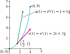
Solution (a) The velocity, acceleration, and speed are \begin{eqnarray*} \mathbf{v}(t)&\;=\;&\mathbf{r}^{\prime} (t)=\dfrac{d}{dt}\left( \dfrac{1}{2} t^{2}+t\right) \mathbf{i}+\dfrac{d}{dt}t^{3}\mathbf{j}=(t+1)\mathbf{i}+3t^{2} \mathbf{j} \\[6pt] \mathbf{a}(t)&\;=\;&\mathbf{r}^{\prime \prime} (t)=\dfrac{d}{dt}\mathbf{r^{\prime} } ( t)\;=\;\dfrac{d}{dt}(t+1)\mathbf{i}+\dfrac{d}{dt}3t^{2}\mathbf{j=i} +6t\mathbf{j} \\[6pt] v(t)&\;=\;&\left\Vert \mathbf{v}(t)\right\Vert\;=\;\sqrt{( t+1) ^{2}+( 3t^{2}) ^{2}}=\sqrt{9t^{4}+t^{2}+2t+1} \end{eqnarray*}
At t=1, the velocity is \mathbf{v}(1)=\mathbf{r}^{\prime} (1)=2\mathbf{i}+3\mathbf{j} and the acceleration is \mathbf{a}(1)=\mathbf{r}^{\prime \prime}(1)=\mathbf{i}+6\mathbf{j}. Figure 25 illustrates the graph of \mathbf{r}=\mathbf{r}( t), \mathbf{v}(1), and \mathbf{a}(1).
786
(b) The velocity, acceleration, and speed of the particle are \begin{eqnarray*} \mathbf{v}(t)&\;=\;&\mathbf{r}^{\prime} (t)=\dfrac{d}{dt}t\mathbf{i}+\dfrac{d}{dt} t^{2}\mathbf{j}+\dfrac{d}{dt}t^{3}\mathbf{k}=\mathbf{i}+2t\mathbf{j}+3t^{2} \mathbf{k} \\[12pt] \mathbf{a}(t)&\;=\;&\mathbf{r}^{\prime \prime} (t)=\dfrac{d}{dt}\mathbf{r^{\prime} } ( t)\;=\;\dfrac{d}{dt}\mathbf{i}+\dfrac{d}{dt}( 2t) \mathbf{j}+\dfrac{d}{dt}( 3t^{2}) \mathbf{k}=2\mathbf{j}+6t \mathbf{k} \\[12pt] v(t)&\;=\;&\left\Vert \mathbf{v}(t)\right\Vert\;=\;\sqrt{1^{2}+( 2t) ^{2}+( 3t^{2}) ^{2}}=\sqrt{1+4t^{2}+9t^{4}} \end{eqnarray*}
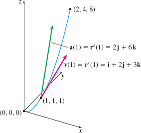
At t=1, the velocity is \mathbf{v}(1)=\mathbf{i}+2\mathbf{j}+3\mathbf{k} and the acceleration is \mathbf{a}(1)=2\mathbf{j}+6\mathbf{k}. See Figure 26.
NOW WORK
EXAMPLE 2Finding the Force Acting on a Particle Moving Along an Ellipse
The position of a particle of mass m that is moving along an ellipse with a constant angular speed \omega is given by the vector function \begin{equation*} \mathbf{r}(t)=A\cos ( \omega t) \mathbf{i}+B\sin ( \omega t) \mathbf{j}\qquad 0\leq t\leq 2\pi \end{equation*}
Find the force \mathbf{F} acting on the particle at any time t. Graph \mathbf{r}=\mathbf{r}( t) and \mathbf{F}=\mathbf{F}( t) .
Solution To find the force \mathbf{F}, we use Newton's Second Law of Motion, \mathbf{F}=m\mathbf{a}. We begin by finding the acceleration \mathbf{a} of the particle. \begin{eqnarray*} \mathbf{r}(t)&\;=\;&A\cos ( \omega t) \mathbf{i}+B\sin ( \omega t) \mathbf{j} \\[3pt] \mathbf{v}(t)&\;=\;&\mathbf{r^{\prime} }(t)=-A\omega \sin ( \omega t) \mathbf{i}+B\omega \cos ( \omega t) \mathbf{j} \\[3pt] \mathbf{a}(t)&\;=\;&\mathbf{r^{\prime \prime} }(t)=-A\omega ^{2}\cos ( \omega t) \mathbf{i}-B\omega ^{2}\sin ( \omega t) \mathbf{j} =-\omega ^{2}\mathbf{r}(t) \end{eqnarray*}
Then, by Newton's Law, \begin{equation*} \mathbf{F}(t)=m\mathbf{a}(t)=-m\hbox{ }\omega ^{2}\mathbf{r}(t) \end{equation*}
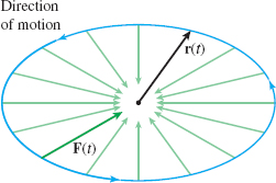
The direction of the force vector \mathbf{F} is opposite to that of the vector \mathbf{r} at any time t, as shown in Figure 27.
NOTE
The force \mathbf{F} acting on the particle in Example 2 is directed toward the center of the ellipse at a time t. Because of this, it is called a centripetal (center-seeking) force.
NOW WORK
EXAMPLE 3Finding the Position, Velocity, and Acceleration of a Particle Moving Along a Circle
(a) Find the position \mathbf{r}=\mathbf{r}( t) of a particle that moves counterclockwise along a circle of radius R with a constant speed v_{0}.
(b) Find the velocity and acceleration of the particle.
(c) Find the magnitude of the acceleration.
Solution For convenience, we place the circle of radius R in the xy-plane, with its center at the origin, and assume that at time t=0 the particle is on the positive x-axis.
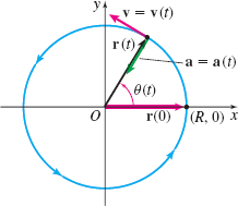
(a) The particle is moving counterclockwise along the circle, as shown in Figure 28. If \theta (t) is the angle between the positive x-axis and the position vector of the particle \mathbf{r}= \mathbf{r}(t), then the vector \mathbf{r=r}( t) is \begin{equation*} \mathbf{r}(t)=R \cos [\theta (t)]{\bf i}+R\;\sin [\theta (t)]{\bf j}\tag{1} \end{equation*}
787
Notice that \mathbf{r}( 0)\;=\;R\mathbf{i}, as required. Also for the motion to be counterclockwise, the function \theta\;=\;\theta ( t) must be increasing.
(b) The velocity \mathbf{v} of the particle is \begin{equation*} \mathbf{v}(t)=\frac{d\mathbf{r}}{dt}=-R\;\sin [\theta (t)]\frac{d\theta }{dt} \mathbf{i}+R\;\cos [\theta (t)]\frac{d\theta }{dt}\mathbf{j}\qquad \color{#0066A7}{\hbox{Use the Chain Rule.}} \end{equation*}
and the speed v of the particle is \begin{eqnarray*} v(t)&=&\left\Vert \mathbf{v}(t)\right\Vert\;=\;\sqrt{R^{2}\sin ^{2}[\theta (t)]\left( \frac{ d\theta }{dt}\right) ^{2}+R^{2}\cos ^{2}[\theta (t)]\left( \frac{d\theta }{dt} \right) ^{2}}\\[6pt] &=&\sqrt{R^{2}\!\left( \frac{d\theta }{dt}\right) ^{2}}=R\left\vert \frac{d\theta }{dt}\right\vert \end{eqnarray*}
Since we know the speed is constant, v(t)=v_{0}. Also, since the function \theta\;=\;\theta ( t) is increasing, \dfrac{d\theta }{dt}>0. As a result, \begin{eqnarray*} v_{0}&=&R\frac{d\theta }{dt} \\[4pt] \frac{d\theta }{dt}&=&\frac{v_{0}}{R} \end{eqnarray*}
Since \dfrac{d\theta }{dt} is the rate at which the angle \theta is changing, the quantity \dfrac{v_{0}}{R} is the angular speed \omega of the particle. That is, \begin{equation*} \frac{d\theta }{dt}=\omega \end{equation*}
We solve this differential equation, using \theta ( 0)\;=\;0 as the initial condition. \begin{eqnarray*} d\theta &=&\omega dt \\[3pt] \theta ( t) &=&\omega t+k \\[3pt] \theta ( 0) &=&k=0 \end{eqnarray*}
So, \theta (t)=\omega t. Now substitute \theta (t)=\omega t into the vector function \mathbf{r=r}( t) [statement (1)] to obtain \begin{equation*} \mathbf{r}(t)=R\;\cos ( \omega t) \mathbf{i}+R\;\sin ( \omega t) \mathbf{j} \end{equation*}
Then the velocity \mathbf{v} and acceleration \mathbf{a} of the particle are \begin{eqnarray*} \mathbf{v}\;=\;\mathbf{v}(t) &=& -R\omega \sin ( \omega t) \mathbf{i} +R\omega \cos ( \omega t) \mathbf{j} \\[3pt] \mathbf{a}\;=\;\mathbf{a}(t) &=& -R\omega ^{2}\cos ( \omega t) \mathbf{i }-R\omega ^{2}\sin ( \omega t) \mathbf{j}=-\omega ^{2}\left[ R\;\cos ( \omega t) \mathbf{i}+R\;\sin ( \omega t) \mathbf{ j}\right]\\[3pt] &=&-\omega ^{2}\mathbf{r}(t) \end{eqnarray*}
(c) Since \omega=\dfrac{v_{0}}{R}, the magnitude of the acceleration is \begin{equation*} \bbox[5px, border:1px solid black, #F9F7ED] {\left\Vert \mathbf{a}(t)\right\Vert\;=\;\omega ^{2}\left\Vert \mathbf{r}(t)\right\Vert\;=\;\omega ^{2}R=\dfrac{v_{0}^{2}}{R}}\tag{2} \end{equation*}
NOW WORK
Observe that although the speed of the particle in Example 3 is constant, its velocity \mathbf{v} is not. Furthermore, the direction of the acceleration is opposite that of the vector \mathbf{r} and is directed toward the center of the circle. By Newton's Second Law of Motion, \mathbf{F}=m\mathbf{a}, so the force vector \mathbf{F} is another example of a centripetal force.
788
NOTE
Near-Earth orbits are above 100 miles (out of Earth's atmosphere) up to an altitude of approximately 15{,}000 miles.
EXAMPLE 4Finding the Speed Required for a Near-Earth Circular Orbit
Find the speed required to maintain a satellite in a near-Earth circular orbit. (The gravitational attraction of other bodies is ignored.)
Solution Let R be the distance of a satellite from the center of Earth. Then from (2), the magnitude of the acceleration of the satellite whose motion is circular is \begin{equation*} \left\Vert \mathbf{a}(t)\right\Vert\;=\;\dfrac{v_{0}^{2}}{R} \end{equation*}
For the satellite to remain in orbit, the magnitude of the acceleration \left\Vert \mathbf{a}(t)\right\Vert of the satellite at any time t must equal g, the acceleration due to gravity for Earth. As a result, \begin{eqnarray*} \frac{v_{0}^{2}}{R}&\;=\;&g \\[3pt] v_{0}&\;=\;&\sqrt{gR} \end{eqnarray*}
The speed v_{0} required to maintain a near-Earth circular orbit is \begin{equation*} \bbox[5px, border:1px solid black, #F9F7ED] {v_{0}=\sqrt{gR}} \end{equation*}
where R is the distance of the satellite from the center of Earth and g is the acceleration due to gravity.
NOTE
The acceleration due to gravity at near-Earth orbits is somewhat less than g ≈ 32.2 \enspace \textrm{ft/s}^{2} ≈ 79{,}036 \enspace \textrm{mi/h}^{2}, the acceleration due to gravity at Earth's surface.
For example, the speed required of a communications satellite whose circular orbit must be 4500 mi from the center of Earth is \begin{equation*} v_{0}=\sqrt{(79{,}036)(4500)}\approx 18{,}859 \enspace \textrm{mi/h} \end{equation*}
NOW WORK
EXAMPLE 5Finding the Frictional Force Necessary to Prevent Skidding
A motorcycle with a mass of 150 kg is driven at a constant speed of 120 km/h on a circular track whose radius is 100 m. To keep the motorcycle from skidding, what frictional force must be exerted by the track on the tires?
Solution By Newton's Second Law of Motion, the force \mathbf{F} required to keep an object of mass m traveling along a curve traced out by \mathbf{r}=\mathbf{r}(t) is \mathbf{F}=m\mathbf{a}. The magnitude of the frictional force exerted by the tires must therefore equal \begin{equation*} \left\Vert \mathbf{F}\right\Vert\;=\;m\left\Vert \mathbf{a}\right\Vert \end{equation*}
In this example, the motion is circular. So, using (2), we have \begin{eqnarray*} &&\left\Vert \mathbf{F}\right\Vert\;=\;m\left( \frac{v_{0}^{2}}{R}\right)\;=\;150\enspace \textrm{kg} \left[\dfrac{\left( 120 \enspace \textrm{km/h}\right)^{2}}{100\enspace \textrm{m}}\right]\quad\,\color{#0066A7}{\underset{{\hbox{$\uparrow$}} }{=}} ( 150) ( 144) \left(\dfrac{1000^{2}}{3600^{2}}\right) \dfrac{\textrm{kg}\,{\cdot}\,\textrm{m}}{\textrm{s}^{2}} \approx 1667\ \enspace \textrm{N}\\[-16.1pt] &&\quad \quad \quad \quad \quad \quad \quad \quad \quad \quad \quad \quad \quad \quad \quad \quad \quad \quad \quad \color{#0066A7}{\hbox{1 h = 3600s}} \end{eqnarray*}
The track must exert a force of magnitude 1667 N or greater to prevent skidding.
NOTE
The SI unit of force is the newton (\textrm{N}): \textrm{N}=\dfrac{\textrm{kg}\,{\cdot}\,\textrm{m}}{\textrm{s}^{2}}.
NOW WORK
2 Express the Acceleration Vector Using Tangential and Normal ComponentsPrinted Page 788
To continue our investigation of the motion of a particle, we show that the acceleration vector \mathbf{a} lies in the plane determined by the unit tangent vector \mathbf{T} and the principal unit normal vector \mathbf{N}.
789
RECALL
The unit tangent vector is \mathbf{T}( t)\;=\;\dfrac{\mathbf{r}^{\prime} ( t) }{\left\Vert \mathbf{r}^{\prime} ( t) \right\Vert }.
Consider a particle whose motion is along a smooth curve C traced out by a twice differentiable vector function \mathbf{r}=\mathbf{r}(t). The velocity vector \mathbf{v}(t)=\mathbf{r}^{\prime} (t) can be expressed in terms of the unit tangent vector \mathbf{T}(t) of C as follows: \begin{equation*} \bbox[5px, border:1px solid black, #F9F7ED] {\mathbf{v}(t)\;=\;\mathbf{r}^{\prime} (t)\;=\;\left\Vert \mathbf{r}^{\prime} (t)\right\Vert \mathbf{T}(t)\;=\;\left\Vert \mathbf{v}(t)\right\Vert \mathbf{T}(t)\;=\;v(t)\mathbf{T} (t)}\tag{3} \end{equation*}
where v(t)\;=\;\left\Vert \mathbf{v}(t)\right\Vert is the speed of the particle
By differentiating \mathbf{v=v}( t), we obtain the acceleration vector \mathbf{a=a}( t) \mathbf{.} \begin{equation*} \mathbf{a}=\mathbf{a}(t)=\dfrac{d}{dt}\mathbf{v}(t)=\frac{d}{dt}[v(t)\mathbf{ T}(t)]=v^{\prime} (t)\mathbf{T}(t)+v(t)\mathbf{T}^{\prime} (t)\ \end{equation*}
RECALL
The principal unit normal vector is \mathbf{N} ( t)\;=\;\dfrac{\mathbf{T}^{\prime} ( t) }{\left\Vert \mathbf{T}^{\prime} ( t) \right\Vert }.
Since \mathbf{T}^{\prime} ( t)\;=\;\left\Vert \mathbf{T}^{\prime} ( t) \right\Vert \mathbf{N}( t), \ \mathbf{a}( t) can be written as \begin{equation*} \mathbf{a}(t)=v^{\prime} (t)\mathbf{T}(t)+v(t)\left\Vert \mathbf{T}^{\prime} (t)\right\Vert \mathbf{N}(t)\tag{4} \end{equation*}
Recall that the curvature \kappa of a curve C traced out by \mathbf{r}=\mathbf{r}( t) can be expressed as \kappa\;=\;\dfrac{\left\Vert \mathbf{T}^{\prime} ( t) \right\Vert }{\left\Vert \mathbf{r}^{\prime} ( t) \right\Vert }, so \begin{equation*} \left\Vert \mathbf{T}^{\prime} ( t) \right\Vert\;=\;\left\Vert \mathbf{r}^{\prime} ( t) \right\Vert \kappa\;=\;v( t) \kappa \tag{5} \end{equation*}
Combining (4) and (5), we have \begin{equation*} \mathbf{a}( t)\;=\;v^{\prime} ( t) \mathbf{T}( t) +\left[ v( t) \right] ^{2}\kappa \mathbf{N}( t) \end{equation*}
THEOREM The Acceleration Vector Expressed Using T and N
The acceleration vector \mathbf{a=a}(t) of a particle moving along a smooth curve C traced out by a twice differentiable vector function \mathbf{r}=\mathbf{r}(t) lies in the plane formed by the unit tangent vector \mathbf{T}(t) and the principal unit normal vector \mathbf{N}(t) to C. Moreover, \begin{equation*} \bbox[5px, border:1px solid black, #F9F7ED] {\mathbf{a}(t)=v^{\prime} (t)\mathbf{T}(t)+[ v(t)] ^{2}\kappa \mathbf{N}(t)}\tag{6} \end{equation*} where v( t) is the speed of the particle and \kappa is the curvature of the curve C traced out by \mathbf{r}=\mathbf{r}( t).
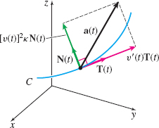
See Figure 29.
The acceleration vector \begin{equation*} \mathbf{a}(t)=\underset{\color{#0066A7}{\hbox{tangential}}\;\\{} \color{#0066A7}{\hbox{component}}}{ \underbrace{v^{\prime} (t)}}\mathbf{T}(t)+\underset{\color{#0066A7}{\quad \hbox{normal }}\\{} \color{#0066A7}{\hbox{component}}}{\underbrace{[ v(t)] ^{2}\kappa }}\mathbf{N }(t) \end{equation*}
has a tangential component, denoted by a_{\mathbf{T}}, and a normal component, denoted by a_{\mathbf{N}}, namely \begin{equation*} \bbox[5px, border:1px solid black, #F9F7ED]{ a_{\mathbf{T}}=v^{\prime }(t)=\dfrac{dv}{dt}\qquad a_{\mathbf{N}}=[ v(t)] ^{2}\kappa} \end{equation*}
Then the acceleration vector can be written as \begin{equation*} \bbox[5px, border:1px solid black, #F9F7ED] {\mathbf{a}(t)=a_{\mathbf{T}}\mathbf{T}(t)+a_{\mathbf{N}}\mathbf{N}(t)} \end{equation*}
Physically, a_{\mathbf{T}} gives the amount of acceleration in the direction of the tangent \mathbf{T}, and a_{\mathbf{N}} gives the amount of acceleration in the direction of the normal \mathbf{N}. For example, if the motion has constant speed [so v^{\prime} ( t)\;=\;0], then the acceleration occurs in the direction of the normal and has no tangential component. In this case, the force \mathbf{F} causing the motion is also in the direction of the normal (\mathbf{F}=m\mathbf{a}).
790

EXAMPLE 6Finding the Tangential and Normal Components of Acceleration for an Elliptical Path
Find the tangential component a_{\mathbf{T}} and normal component a_{\mathbf{N}} of the acceleration of a particle moving along the ellipse \begin{equation*} \mathbf{r}(t)=3\sin t\mathbf{i}+4\cos t\mathbf{j}\quad 0\leq t\leq 2\pi \end{equation*}
Graph the ellipse, showing \mathbf{a}=\mathbf{a}( t), a_{\mathbf{T}}, and a_{\mathbf{N}} when t=0, \dfrac{\pi }{4}, and \dfrac{\pi }{2}.
Solution We begin by finding the velocity, speed, and acceleration of the particle. \begin{eqnarray*} \mathbf{v}(t)&=&\mathbf{r}^{\prime} (t)=3\cos t\mathbf{i}-4\sin t\mathbf{j}\\[3pt] v(t)&=&\left\Vert \mathbf{v}(t)\right\Vert\;=\;\sqrt{(3\cos t)^{2}+(-4\sin t)^{2}}=\sqrt{9\cos ^{2}t+16\sin ^{2}t} \\[3pt] \mathbf{a}(t)&=&\mathbf{r}^{\prime \prime} (t)=-3\sin t\mathbf{i}-4\cos t \mathbf{j} \end{eqnarray*}
The tangential component of the acceleration is \begin{eqnarray*} a_{\mathbf{T}}=v^{\prime} ( t) &=&\dfrac{d}{dt}\sqrt{9\cos ^{2}t+16\sin ^{2}t}\\[3pt] &=&\dfrac{1}{2}( 9\cos ^{2}t+16\sin ^{2}t) ^{-1/2}[ 18\cos t ( -\!\sin t) +32\sin t (\cos t)]\\[3pt] &=&\frac{7\sin t\cos t}{\sqrt{9\cos ^{2}t+16\sin ^{2}t}} \end{eqnarray*}
To find the normal component of the acceleration, we need to find the curvature \kappa of \mathbf{r}=\mathbf{r}( t). \begin{eqnarray*} \kappa &=&\dfrac{\left\Vert \mathbf{r}^{\prime} ( t) \times \mathbf{r} ^{\prime \prime} ( t) \right\Vert }{\left\Vert \mathbf{r}^{\prime} ( t) \right\Vert ^{3}}=\dfrac{ \left\| \bbox[5px]{\begin{vmatrix} {\bf i} & {\bf j} & {\bf k}\\ {3 \cos t} & {-4 \sin t} & {0} \\ {-3 \sin t} & {-4 \cos t} & {0} \end{vmatrix}} \right\| }{( 9\cos ^{2}t+16\sin ^{2}t) ^{3/2}}=\dfrac{\left\vert\!-\!12\cos^{2}t-12\sin ^{2}t\right\vert }{( 9\cos ^{2}t+16\sin ^{2}t) ^{3/2} }\\[3pt] &=&\dfrac{12}{( 9\cos ^{2}t+16\sin ^{2}t) ^{3/2}} \end{eqnarray*}
Then \begin{equation*} a_{\mathbf{N}}=v^{2}( t) \kappa\;=\;( 9\cos ^{2}t+16\sin ^{2}t) \dfrac{12}{( 9\cos ^{2}t+16\sin ^{2}t) ^{3/2}}=\frac{ 12}{\sqrt{9\cos ^{2}t+16\sin ^{2}t}} \end{equation*}
The motion of the particle on the ellipse starts at \mathbf{r}(0)=4\mathbf{j}. As t increases, x( t)\;=\;3 \sin t increases and y( t)\;=\;4\cos t decreases, so the motion of the particle is clockwise.
At t=0, \begin{equation*} \mathbf{a}( 0)\;=\;-3( 0) \mathbf{i}-4( 1) \mathbf{j}=-4\mathbf{j}\quad a_{\mathbf{T}}=\dfrac{7( 0) ( 1) }{3}=0\quad a_{\mathbf{N}}=\dfrac{12}{3}=4 \end{equation*}
At t=\dfrac{\pi }{4}, \mathbf{r}\left( \dfrac{\pi }{4}\right)\;=\;\dfrac{3\sqrt{2}}{2}\mathbf{i}+2\sqrt{2}\mathbf{j}, and \begin{equation*} \mathbf{a}\left( \dfrac{\pi }{4}\right)\;=\;-\dfrac{3\sqrt{2}}{2}\mathbf{i}-2 \sqrt{2}\mathbf{j}\quad a_{\mathbf{T}}=\dfrac{7\sqrt{2}}{10}\quad a_{\mathbf{N}}=\dfrac{12\sqrt{2}}{5} \end{equation*}
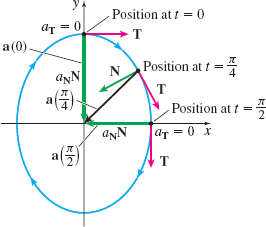
At t=\dfrac{\pi }{2}, \mathbf{r}\left( \dfrac{\pi }{2}\right)\;=\;3\mathbf{i}+4( 0) \mathbf{j}=3\mathbf{i}, and \begin{equation*} \mathbf{a}\left( \dfrac{\pi }{2}\right)\;=\;-3( 1) \mathbf{i} -4( 0) \mathbf{j=}-\!3\mathbf{i}\quad a_{\mathbf{T} }=0\quad a_{\mathbf{N}}=\dfrac{12}{4}=3 \end{equation*}
See Figure 30.
NOW WORK
791
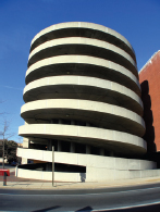
EXAMPLE 7Analyzing the Acceleration of a Car
A car on the ramp of a multistory parking garage travels along a curve traced out by \mathbf{r}( t)\;=\;10\cos t\mathbf{i}+10\sin t\mathbf{j}+3t\mathbf{k}, where t is the time in hours and distance is in miles. Find the tangential component a_{\mathbf{T}} and normal component a_{\mathbf{N}} of the acceleration of the car. What are the magnitude and direction of the force on the driver?
Solution We begin by finding the velocity \mathbf{v}, speed v , and acceleration \mathbf{a} of the car. \begin{eqnarray*} \mathbf{v}(t)&\;=\;&\mathbf{r}^{\prime} (t)=\dfrac{d}{dt}( 10\cos t) \mathbf{i}+\dfrac{d}{dt}( 10\sin t) \mathbf{j}+\dfrac{d}{dt} ( 3t) \mathbf{k}=-10\sin t\mathbf{i}+10\cos t\mathbf{j+}3 \mathbf{k} \\[6pt] v(t)&\;=\;&\left\Vert \mathbf{v}(t)\right\Vert\;=\;\left\Vert \mathbf{r}^{\prime} (t)\right\Vert\;=\;\sqrt{(-10\sin t)^{2}+(10\cos t)^{2}+9}=\sqrt{109}\approx 10.440 \enspace \textrm{mi/h}\\[6pt] \mathbf{a}(t)&\;=\;&\mathbf{r^{\prime\prime}} (t)=\dfrac{d}{dt}\mathbf{v}(t)= -10\cos t\mathbf{i}-10\sin t\mathbf{j } \end{eqnarray*}
Since the speed is constant, the tangential component of acceleration a_{ \mathbf{T}} is \begin{eqnarray*} a_{\mathbf{T}}=\dfrac{dv}{dt}=0 \end{eqnarray*}
The normal component of acceleration a_{\mathbf{N}} is 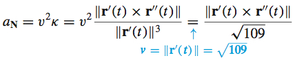
Since, \begin{equation*} \mathbf{r}^{\prime} (t)\times \mathbf{r}^{\prime \prime} (t)= \left|\begin{array}{c@{\quad}c@{\quad}c} \mathbf{i} & \mathbf{j} & \mathbf{k} \\[3pt] -10\sin t & 10\cos t & 3 \\[3pt] -10\cos t & -10\sin t & 0 \end{array}\right| =30\sin t\mathbf{i}-30\cos t\mathbf{j}+100\mathbf{k} \end{equation*}
the normal component is \begin{eqnarray*} a_{\mathbf{N}}&=&\frac{\left\Vert 30\sin t\mathbf{i}-30\cos t\mathbf{j}+100 \mathbf{k}\right\Vert }{\sqrt{109}}=\dfrac{\sqrt{900\sin ^{2}t+900\cos ^{2}t+10000} }{\sqrt{109}}\\[4pt] &=&\dfrac{\sqrt{10900}}{\sqrt{109}}=10 \end{eqnarray*}
As the car travels on the ramp at a constant speed, the force \mathbf{F}=m\mathbf{a}\;=\;ma_{\mathbf{N}} \mathbf{N}\;=\;10 m \mathbf{N}
pulls the car and driver toward the center of the ramp, with a magnitude about 10 times the mass of the car.
NOW WORK
Application: The UVW-Axes in Orbital Mechanics
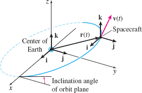
A spacecraft in orbit about Earth follows a curve in space, which is modeled as the graph of a vector function of time t. The spacecraft carries a gyroscope whose three axes remain fixed in direction throughout time and are aligned with the \mathbf{i},~\mathbf{j},~\mathbf{k} unit vectors of the xyz-coordinate system. The xyz-coordinate system has its origin at the center of Earth, providing the same basic frame of reference for both Earth-bound observers and the spacecraft. See Figure 31.
Suppose the position of the spacecraft is given by the vector function \begin{equation*} \mathbf{r}(t)=x(t)\mathbf{i}+y(t)\mathbf{j}+z(t)\mathbf{k} \end{equation*}
Then the velocity vector \mathbf{v=v}( t) is tangent to the orbit: \mathbf{v}(t)=\mathbf{r}^{\prime} (t).
792
If Earth is taken to have all its mass concentrated at the center, then the laws of Kepler and Newton tell us that any orbit remains in a fixed plane containing the center. Furthermore, a closed orbit describes an ellipse (or circle) in that plane with Earth's center at one of the foci.
The UVW system of axes is an orthogonal set of unit vectors \mathbf{i}_{ \mathbf{U}}(t),~\mathbf{i}_{\mathbf{V}}(t),~\mathbf{i}_{\mathbf{W}}(t) that are “attached“ to the spacecraft's orbit at each point. This set of vectors is particularly useful in manned spacecraft, since it corresponds to the axes of yaw, roll, and pitch customarily used in airplanes flying over the surface of Earth. These time-dependant unit vectors are defined as \begin{equation} \mathbf{i}_{\mathbf{U}}=\frac{\mathbf{r}}{\left\Vert \mathbf{r}\right\Vert },\qquad \mathbf{i}_{\mathbf{W}}=\frac{\mathbf{r}\times \mathbf{v}}{\left\Vert \mathbf{r} \times \mathbf{v}\right\Vert },\qquad \mathbf{i}_{\mathbf{V}}=\mathbf{i}_{\mathbf{W} }\times \mathbf{i}_{\mathbf{U}}\tag{7} \end{equation}
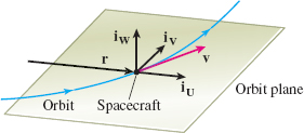
Notice that \mathbf{i}_{\mathbf{U}}(t) lies in the orbit plane and points radially outward. Since both \mathbf{r} and \mathbf{v} are vectors in the orbit plane and \mathbf{r}\times \mathbf{v} is orthogonal to both \mathbf{r} and \mathbf{v}, the vector \mathbf{i}_{\mathbf{W}}(t) is normal to the orbit plane. The vector \mathbf{i}_{\mathbf{V}}(t) completes the set of axes and lies in the orbit plane. See Figure 32.
EXAMPLE 8Finding the UVW-Axes of an Orbit
A satellite in a circular orbit intersects the x-axis and is inclined to the xy-plane at an angle of 30{{}^\circ}. Suppose the orbit has a radius a, and the motion has angular speed \omega . Then the position of the satellite at time t is \begin{equation*} \mathbf{r}(t)=a\!\left( \cos ( \omega t) \mathbf{i}+\frac{\sqrt{3}}{ 2}\sin ( \omega t) \mathbf{j}+\frac{1}{2}\sin ( \omega t) \mathbf{k}\right) \end{equation*}
The velocity vector \mathbf{v} is \begin{equation*} \mathbf{v}(t)=\mathbf{r}^{\prime} (t)=a\omega \!\left( -\!\sin ( \omega t) \mathbf{i}+\frac{\sqrt{3}}{2}\cos ( \omega t) \mathbf{j}+ \frac{1}{2}\cos ( \omega t) \mathbf{k}\right) \end{equation*}
In this case, using (7), the UVW system of axes is \begin{array}{rcl@{\qquad}rcl} \mathbf{i}_{\mathbf{U}}&=&\cos ( \omega t) \mathbf{i}+\frac{\sqrt{3}}{2}\sin ( \omega t) \mathbf{j}+\frac{1}{2}\sin ( \omega t) \mathbf{k} & \color{#0066A7}{\mathbf{i}_{\mathbf{U}}}&{\color{#0066A7}=}&\color{#0066A7}{\tfrac{\mathbf{r}}{\left\Vert \mathbf{r}\right\Vert }}\\ \mathbf{i}_{\mathbf{W}}&=&-\frac{1}{2}\mathbf{j}+\frac{\sqrt{3}}{2}\mathbf{k}& \color{#0066A7}{\mathbf{i}_{\mathbf{W}}}&{\color{#0066A7}=}& \color{#0066A7}{\tfrac{\mathbf{r}\times \mathbf{v}}{\left\Vert \mathbf{r}\times \mathbf{v}\right\Vert }}\\ \mathbf{i}_{\mathbf{V}}&\;=\;&-\sin ( \omega t) \mathbf{i}+\frac{ \sqrt{3}}{2}\cos ( \omega t) \mathbf{j}+\frac{1}{2}\cos ( \omega t) \mathbf{k} & \color{#0066A7}{\mathbf{i}_{\mathbf{V}}}&{\color{#0066A7}=}&\color{#0066A7}{\mathbf{i}_{\mathbf{W}}\times \mathbf{i}_{\mathbf{U}}} \end{array}
The directions of the onboard gyroscope axes UVW are now expressed in terms of \mathbf{i}, \mathbf{j}, and \mathbf{k}.