15.5 Green’s TheoremPrinted Page 1008
In this section, we investigate an amazing theorem, known as Green’s Theorem, that relates the value of a line integral along a simple closed curve C in the plane to a double integral over the region R enclosed by C.
ORIGINS
George Green (1793–1841) was a miller and self-taught mathematician who also worked with applications in electricity, magnetism, and fluid flow.
Green’s Theorem may be stated in several ways, but the most common form is the following: \bbox[5px, border:1px solid black, #F9F7ED]{\bbox[#FAF8ED,5pt]{ \oint_{C}(P\,dx+Q\,dy)=\iint\limits_{R}\left( \dfrac{ \partial Q}{\partial x}-\dfrac{\partial P}{\partial y}\right) dx\,dy }}
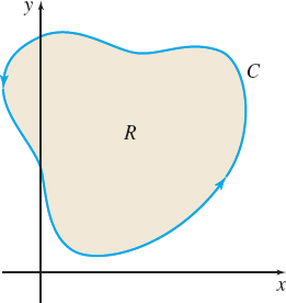
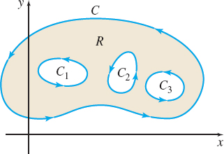
The plane curve C is the boundary of the region R, and the symbol \oint indicates that the simple closed curve C is to be traversed in a counterclockwise direction. That is, the region R always lies to the left as one moves along the curve, as shown in Figure 31.
The equality \oint_{C}(P\,dx+Q\,dy)=\iint\limits_{R}\left( \dfrac{\partial Q }{\partial x}-\dfrac{\partial P}{\partial y}\right) dx\,dy requires two assumptions:
- The functions P and Q have continuous first-order partial derivatives at each point in the region R.
- The curve C is a piecewise-smooth, simple closed curve, and the region R is both simply connected and closed.
The advantage of using Green’s Theorem is that it can be used to transform line integrals into double integrals and vice versa, allowing us the opportunity to find the easier of the two.
RECALL
A region R is closed if it contains all its boundary points.
THEOREM Green’s Theorem
Let C be a piecewise-smooth, simple closed curve with a counter clockwise orientation and let R be the simply connected, closed region consisting of C and its interior. Let the functions P and Q have continuous first-order partial derivatives on some open region that contains R. Then \bbox[5px, border:1px solid black, #F9F7ED]{\bbox[#FAF8ED,5pt]{ \oint_{C}(P\,dx+Q\,dy)=\iint\limits_{R}\left( \dfrac{\partial Q}{\partial x}-\dfrac{\partial P}{\partial y}\right) dx\,dy}}
where the line integral is taken around C in the counterclockwise direction.
NEED TO REVIEW?
x-simple and y-simple regions are discussed in Section 14.2, pp. 913 and 915.
We prove Green’s Theorem only for regions that are both x-simple and y-simple.
1009
Proof
It is sufficient to show that \oint_{C}P(x,y)\,dx=-\iint\limits_{R}\dfrac{\partial P}{\partial y}\,dx\,dy \qquad \hbox{and}\qquad \oint_{C}Q(x,y)\,dy=\iint\limits_{R}\dfrac{\partial Q}{\partial x}\,dx\,dy
since the result follows from adding these two equations.
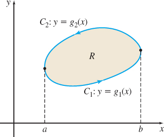
Suppose the region R is both x-simple and y-simple. Then since it is x-simple as shown in Figure 32, the boundary of R consists of two smooth curves, C_{1}: y=g_{1}(x) and C_{2}: y=g_{2}(x), where g_{1}(x)\leq g_{2}(x), a\leq x\leq b.
To show \oint_{C}P(x,y)\,dx=-\iint\limits_{R}\dfrac{\partial P}{\partial y} \,dx\,dy, we begin with the double integral. Since R is x-simple, by Fubini’s Theorem, we have \begin{eqnarray*} -\iint\limits_{R}\dfrac{\partial P}{\partial y}\,dx\,dy& =&-\int_{a}^{b}\left[\int_{g_{1}(x)}^{g_{2}(x)}\dfrac{\partial P}{\partial y}\,dy\right] dx=-\int_{a}^{b}\big[ P(x,y)\big] _{g_{1}(x)}^{g_{2}(x)}\,dx \\ & =&-\int_{a}^{b}[ P(x,g_{2}(x))-P(x,g_{1}(x))]\,dx=\int_{a}^{b}P(x,g_{1}(x))\,dx+\int_{b}^{a}P(x,g_{2}(x))\,dx \\ &=&\int_{C_{1}}P(x,y)\,dx+\int_{C_{2}}P(x,y)\,dx =\oint_{C}P(x,y)\,dx \end{eqnarray*}
To show \oint_{C}Q(x,y)\,dy=\iint\limits_{R}\dfrac{\partial Q}{\partial x} \,dx\,dy, use the fact that the region R is also y-simple. The derivation is left as an exercise (Problem 49).
NEED TO REVIEW?
Fubini’s Theorems are discussed in Section 14.2, pp. 913 and 915.
1 Use Green’s Theorem to Find a Line IntegralPrinted Page 1009
EXAMPLE 1Finding a Line Integral Using Green’s Theorem
Use Green’s Theorem to find the line integral \begin{equation*} \oint_{C}[ ( -2xy+y^{2}) \,dx+x^{2}\,dy] \end{equation*}
where C is the boundary of the region R enclosed by y=4x and y=2x^{2}.
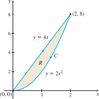
Solution Figure 33 illustrates the curve C and the region R. C is a piecewise-smooth closed curve and R is both simply connected and closed. We let \begin{equation*} P(x,y)=-2xy+y^{2}\qquad \hbox{and}\qquad Q(x,y)=x^{2} \end{equation*}
Since P and Q have continuous first-order partial derivatives in R, we use Green’s Theorem. Then \begin{eqnarray*} \oint_{C}(P\,dx+Q\,dy)& =&\iint\limits_{R}\left( \dfrac{\partial Q}{\partial x }-\dfrac{\partial P}{\partial y}\right) \,dx\,dy \\ \oint_{C}[(-2xy+y^{2})\,dx+x^{2}\,dy]& =&\iint\limits_{R}\left[ \dfrac{ \partial }{\partial x}(x^{2})-\dfrac{\partial }{\partial y}(-2xy+y^{2})\right] \,dx\,dy\\ &=&\iint\limits_{R}(4x-2y)\,dx\,dy \underset{\underset{\color{#0066A7}{R\hbox{ is } x\hbox{-simple}}}{\color{#0066A7}{\uparrow}}} {=} \int_{0}^{2} \int_{2x^{2}}^{4x}(4x-2y)\,dy\,dx \\ & =&\int_{0}^{2}\big[ 4xy-y^{2}\big] _{2x^{2}}^{4x}\,dx = \int_{0}^{2}[(16x^{2}-16x^{2})-(8x^{3}-4x^{4})]\,dx \\ & =&\left[ -2x^{4}+\dfrac{4}{5}x^{5}\right] _{0}^{2}=-32+\dfrac{128}{5}=\dfrac{ -32}{5} \end{eqnarray*}
NOW WORK
1010
The solution found in Example 1 can be verified by finding the line integral directly. Let C_{1} be the curve traced out by y=2x^{2}, 0\leq x\leq 2, and let C_{2} be the curve traced out by y=4x, from 2 to 0. Then \begin{eqnarray*} \oint_{C}[(-2xy+y^{2})\,dx+x^{2}\,dy]&=& \int_{C_{1}}[(-2xy+y^{2})\,dx+x^{2}\,dy]+\int_{C_{2}}[(-2xy+y^{2})\,dx+x^{2} \,dy] \\ &=& \int_{0}^{2}[(-4t^{3}+4t^{4})\,dt+4t^{3}\,dt] \quad\color{#0066A7}{\begin{array}{c} C_{1}: x=t, y=2t^{2}, 0\leq t \leq 2 \\ C_{2}: x=t, y=4t;\hbox{ from } t=2 \hbox{ to } t=0 \end{array}}\\ &&+\,\int_{2}^{0}[(-8t^{2}+16t^{2})\,dt+4t^{2}\,dt]\\ &=& \left[ 4\dfrac{t^{5}}{5}\right] _{0}^{2}+12\left[ \dfrac{t^{3}}{3}\right] _{2}^{0}=\dfrac{128}{5}-32=-\dfrac{32}{5} \end{eqnarray*}
The next example shows that Green’s Theorem can be helpful in finding line integrals that are difficult or impossible to find using the techniques of Section 15.2.
EXAMPLE 2Finding a Line Integral Using Green’s Theorem
Use Green’s Theorem to find the line integral \begin{equation*} \oint_{C}[ ( e^{-x^{2}}+y^{2}) \,dx+( \ln y-x^{2}) \,dy] \end{equation*}
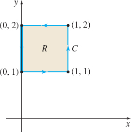
where C is the square illustrated in Figure 34.
Solution Recall that \int e^{-x^{2}}dx cannot be expressed in terms of elementary functions, so finding the integral directly is impossible. Since both the curve C and the region R enclosed by C satisfy the conditions of Green’s Theorem, we use it to find the line integral. If P(x,y)=e^{-x^{2}}+y^{2} and Q(x,y)=\ln y-x^{2} then \dfrac{\partial P}{ \partial y}=2y and \dfrac{\partial Q}{\partial x}=-2x. Since P and Q have continuous first-order derivatives in R, by Green’s Theorem, We have \begin{eqnarray*} &&\oint_{C}[(e^{-x^{2}}+y^{2})\,dx+(\ln y-x^{2})]\,dy =\iint\limits_{R}(-2x-2y)\,dx\,dy \\ &&\hspace{10.4pc}=-2\int_{1}^{2}\int_{0}^{1}(x+y) \,dx\,dy=-2\int_{1}^{2}\left[ \dfrac{x^{2}}{2}+xy\right] _{0}^{1}\,dy \\ &&\hspace{9.1pc}\underset{\color{#0066A7}{R\hbox{ is } y\hbox{-simple}}}{\color{#0066A7}{\uparrow}}\\ &&\hspace{10.4pc}=-2\int_{1}^{2}\left( \dfrac{1}{2}+y\right) dy=-2\left[ \dfrac{1}{2}y+ \dfrac{y^{2}}{2}\right] _{1}^{2}=-4 \end{eqnarray*}
NOW WORK
In Example 2, Green’s Theorem was used to convert a line integral into a double integral because the line integral could not be found. Green’s Theorem is also used to convert double integrals to line integrals when the line integral is easier to integrate. This is often true when finding area.
2 Use Green’s Theorem to Find AreaPrinted Page 1010
Green’s Theorem can be used to express the area A of a region R enclosed by a piecewise-smooth, simple closed curve C as a line integral.
THEOREM Green’s Theorem for Area
If C is a piecewise-smooth, simple closed curve with a counterclockwise orientation, then the area A of the simply connected closed region R enclosed by C is given by \bbox[5px, border:1px solid black, #F9F7ED]{\bbox[#FAF8ED,5pt]{ A=\dfrac{1}{2}\oint_{C}(-y\,dx+x\,dy) }} \tag{1}
1011
Proof
In Green’s Theorem, let P=P(x,y)=-y and Q=Q(x,y)=x. Then \oint_{C}(-y\,dx+x\,dy)=\iint\limits_{R}\left[ \dfrac{\partial }{\partial x} (x)-\dfrac{\partial }{\partial y}(-y)\right] \,dx\,dy=\iint\limits_{R}2\,dx \,dy=2A
RECALL
\iint\limits_{R}\,dx\,dy equals the area of the region R.
In Problem 50, you are asked to show that the area A can also be expressed by the formulas \bbox[5px, border:1px solid black, #F9F7ED]{\bbox[#FAF8ED,5pt] {A=\oint_{C}x\,dy \qquad \hbox{and}\qquad A=\oint_{C}(-y)\,dx }}
EXAMPLE 3Using Green’s Theorem to Find Area
Use Green’s Theorem to find the area of the region enclosed by the ellipse \dfrac{x^{2}}{a^{2}}+\dfrac{y^{2}}{b^{2}}=1\qquad a>0\quad b>0
Solution We express the ellipse using the parametric equations x=a\;\cos t, y=b\;\sin t, 0\leq t\leq 2\pi . Then dx=-a\;\sin t\,dt and dy=b\;\cos t\,dt. Now we use (1) to find the area. \begin{eqnarray*} A& =&\dfrac{1}{2}\oint_{C}(-y\,dx+x\,dy)=\dfrac{1}{2}\int_{0}^{2\pi }[-b\sin t(-a\sin t\,dt)+a\cos t(b\cos t\,dt)] \\ & =&\dfrac{1}{2}\int_{0}^{2\pi }ab(\sin ^{2}t+\cos ^{2}t)\,dt=\dfrac{1}{2}(ab)\int_{0}^{2\pi }dt=\dfrac{1}{2}ab(2\pi )=\pi ab \end{eqnarray*}
NOW WORK
3 Use Green’s Theorem with Multiply-Connected RegionsPrinted Page 1011
For Green’s Theorem to hold, the double integral is found over a simply connected, closed region R formed by a piecewise-smooth, simple closed curve C and its interior. We now consider Green’s Theorem for multiply-connected regions.
A multiply-connected region is any connected region that is not simply connected. We can think of a multiply connected region as a connected region with holes. See Figure 35.
THEOREM Green’s Theorem for Multiply-Connected Regions
Let C_{1}, C_{2}, \ldots , C_{n} be n piecewise-smooth, simple closed curves for which:
- No two curves C_{i} and C_{j}, i\neq j, i, j=1, 2, \ldots , n, intersect.
- Each of the curves C_{i}, i=1, 2, \ldots , n lies in the interior of a piecewise-smooth, simple closed curve C.
- Any curve C_{i} is exterior to every curve C_{j}, i\neq j, i, j=1, 2, \ldots , n.
Let R denote the region consisting of the interior of C and its boundary, less the interior of each of the curves C_{1}, C_{2}, \ldots , C_{n}. Let functions P and Q have continuous first-order partial derivatives throughout R. Then \bbox[5px, border:1px solid black, #F9F7ED]{\bbox[#FAF8ED,5pt]{ \iint\limits_{R}\left( \dfrac{\partial Q}{\partial x}- \dfrac{\partial P}{\partial y}\right) dx\,dy=\oint_{C}(P\,dx+Q\,dy) - \sum\limits_{i=1}^{n}\oint_{C_{i}}(P \,dx+Q\,dy) }}
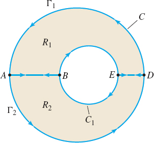
We give the idea of the proof for n=1. As shown in Figure 36, the curve C_{1} is a circle contained within the larger circle C.
Proof
We construct line segments \overline{AB} and \overline{ED} that join the curves C and C_{1}. This decomposes R into two regions R_{1} and R_{2}, with boundaries \Gamma _{1} and \Gamma _{2}, respectively.
1012
Since R_{1} and R_{2} each satisfy the conditions of Green’s Theorem, we have \begin{eqnarray*} \iint\limits_{R}\left( \dfrac{\partial Q}{\partial x}-\dfrac{\partial P}{ \partial y}\right) dx\,dy &=&\iint\limits_{R_{1}}\left( \dfrac{\partial Q}{ \partial x}-\dfrac{\partial P}{\partial y}\right) dx\,dy+\iint\limits_{R_{2}}\left( \dfrac{\partial Q}{\partial x}-\dfrac{ \partial P}{\partial y}\right) dx\,dy \\ &=&\oint_{\Gamma _{1}}(P\,dx+Q\,dy)+\oint_{\Gamma _{2}}(P\,dx+Q\,dy) \\ &=&\left[ \int_{DA}(P\,dx+Q\,dy)+\int_{\overline{AB}}(P\,dx+Q\,dy)+ \int_{BE}(P\,dx+Q\,dy)+\int_{\overline{ED}}(P\,dx+Q\,dy)\right] \\ &&+\left[ \int_{\overline{DE}}(P\,dx+Q\,dy)+\int_{EB}(P\,dx+Q\,dy)+\int_{ \overline{BA}}(P\,dx+Q\,dy)+\int_{AD}(P\,dx+Q\,dy)\right] \end{eqnarray*}
Along the line segments \overline{AB} and \overline{ED}, \int_{\overline{AB}}(P\,dx+Q\,dy)=-\int_{\overline{BA}}(P\,dx+Q\,dy)\quad\hbox{and}\quad \int_{\overline{ED}}(P\,dx+Q\,dy)=-\int_{\overline{DE} }(P\,dx+Q\,dy)
So, \begin{eqnarray*} \iint\limits_{R}\left( \dfrac{\partial Q}{\partial x}-\dfrac{\partial P}{ \partial y}\right) dx\,dy &=&\oint_{C}(P\,dx+Q\,dy)+\oint_{-C_{1}}(P\,dx+Q\,dy) \\ &=&\oint_{C}(P\,dx+Q\,dy)-\oint_{C_{1}}(P\,dx+Q\,dy) \end{eqnarray*}
The next theorem is an important consequence of Green’s Theorem for Multiply Connected Regions.
THEOREM
Let P and Q be functions that have continuous first-order partial derivatives throughout an open, connected set R. Let C_{1} and C_{2} denote two piecewise-smooth, simple closed curves, each lying entirely in R . Suppose the curve C_{1} can be obtained by continuously deforming the curve C_{2} so that all the intermediate deformed curves lie entirely in R. If \dfrac{\partial P }{\partial y}=\dfrac{\partial Q}{\partial x} throughout R, then \bbox[5px, border:1px solid black, #F9F7ED]{\bbox[#FAF8ED,5pt]{ \int_{C_{1}}(P\,dx+Q\,dy)=\int_{C_{2}}(P\,dx+Q\,dy) }}
The significance of this theorem is that it allows us, under the conditions of the theorem, to replace a line integral over a simple closed curve C_{1} that is difficult to find with an easier line integral over the path C_{2}.
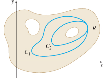
Figure 37 illustrates a set R satisfying the conditions of the theorem, which can be restated informally as follows: If \dfrac{\partial P}{\partial y}=\dfrac{\partial Q}{\partial x} throughout R, then the value of a line integral along a piecewise-smooth, simple closed curve equals the value of the same line integral along any other piecewise-smooth, simple closed curve that is obtained by continuously deforming the original curve, provided all the intermediate deformed curves lie entirely in R.
EXAMPLE 4Using Green’s Theorem to Find a Line Integral
Find \oint_{\!\!\!\!C}\left( \dfrac{-y}{x^{2}+y^{2}}\,dx+\dfrac{x}{x^{2}+y^{2}} \,dy\right) if:
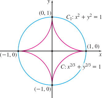
- (a) C is the curve x^{2/3}+y^{2/3}=1, whose orientation is counterclockwise.
- (b) C is any piecewise-smooth, simple closed curve not containing the origin in its interior.
1013
Solution For P=\dfrac{-y}{x^{2}+y^{2}} and Q=\dfrac{x}{ x^{2}+y^{2}}, we have \dfrac{\partial P}{\partial y}=\dfrac{y^{2}-x^{2}}{(x^{2}+y^{2})^{2}}\qquad \hbox{and} \qquad \dfrac{\partial Q}{\partial x}=\dfrac{y^{2}-x^{2}}{(x^{2}+y^{2})^{2}}
Notice that, except at the point (0,0), the partial derivatives \dfrac{ \partial P}{\partial y} and \dfrac{\partial Q}{\partial x} are continuous.
(a) It is difficult to find the line integral along C. Moreover, because x^{2/3}+y^{2/3}=1 contains the point (0,0) in its interior, we cannot use Green’s Theorem as we did in Example 2 to change the line integral to a double integral. However, since \dfrac{ \partial P}{\partial y}=\dfrac{\partial Q}{\partial x} throughout R, we can use a different curve that leads to an easier line integral. For example, suppose we replace x^{2/3}+y^{2/3}=1 by the unit circle C_{1}: x^{2}+y^{2}=1, noting that the conditions required for \int_{C}( P\,dx+Q\,dy) to equal \int_{C_{1}}( P\,dx+Q\,dy) are met. See Figure 38.
On C_{1}, x=\cos \theta, y=\sin \theta, 0\leq \theta \leq 2\pi. Then dx=-\sin \theta d\theta , dy=\cos \theta d\theta, and \begin{eqnarray*} \oint_{C}\left( \dfrac{-y}{x^{2}+y^{2}}\,dx+\dfrac{x}{x^{2}+y^{2}}\,dy\right) &=&\oint_{C_{1}}\left( \dfrac{-y}{x^{2}+y^{2}}\,dx+\dfrac{x}{x^{2}+y^{2}} \,dy\right)\\ &=&\int_{0}^{2\pi }(\sin ^{2}\theta +\cos ^{2}\theta )\,d\theta =2\pi \end{eqnarray*}
(b) In this case, the interior of the curve C does not contain the origin. Since \begin{equation*} \dfrac{\partial P}{\partial y}=\dfrac{\partial Q}{\partial x} \end{equation*}
in the simply connected region R enclosed by C, it follows that \mathbf{ F}=P(x,y)\mathbf{i}+Q(x,y)\mathbf{j} is a conservative vector field. Since C is closed, \oint_{C}\left( \dfrac{-y}{x^{2}+y^{2}}\,dx+\dfrac{x}{x^{2}+y^{2}}\,dy\right)= \oint_{C}\mathbf{F}\,{\bf\cdot}\, d\mathbf{r} =0
NOW WORK
Application of Green’s Theorem to Conservative Vector Fields
In Section 15.3, we proved the following result: If \mathbf{F}=\mathbf{F}(x,y)=P(x,y)\mathbf{i}+Q(x,y)\mathbf{j} is a conservative vector field and the components P and Q have continuous first-order partial derivatives on an open, connected region R, then \dfrac{\partial P}{\partial y}=\dfrac{\partial Q}{\partial x} throughout R.
We now use Green’s Theorem to prove that if R is a simply connected region, then the converse is also true.
THEOREM Converse of the Conservative Vector Field Theorem
Let \mathbf{F}=P(x,y)\mathbf{i}+Q(x,y)\mathbf{j} be a vector field whose components P and Q have continuous first-order partial derivatives throughout an open, simply connected region R. If \dfrac{\partial P}{ \partial y}=\dfrac{\partial Q}{\partial x} throughout R, then \mathbf{F} is a conservative vector field.
To show that \mathbf{F} is a conservative vector field, we only need to show that for any curve C in R, \int_{C}\mathbf{F}\,{\bf\cdot}\, d\mathbf{r} =\int_{C}(P\,dx+Q\,dy) is independent of the path. That is, \int_{C} \mathbf{F}\,{\bf\cdot}\, d\mathbf{r} has the same value for any two piecewise-smooth curves joining a fixed point A in R to an arbitrary point (x,y) in R.
1014
Proof
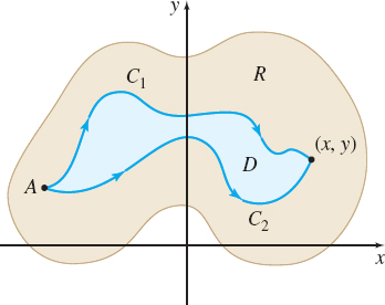
Let C_{1} and C_{2} be two piecewise-smooth curves in R joining A to (x,y). Assume that these curves do not intersect or coincide except at A and (x,y).* The curves C_{1} and C_{2} form the boundary of a region D that is a subset of R, since R is simply connected. See Figure 39.
* This assumption may be relaxed so that the curves C_{1} and C_{2} may sometimes interesect or even coincide in R.
Since the conditions for Green’s Theorem are satisfied on the region D, we have \begin{eqnarray*} \iint\limits_{D}\left( \dfrac{\partial Q}{\partial x}-\dfrac{\partial P}{ \partial y}\right) \,dx\,dy& =&\int_{C_{2}+( -C_{1})}(P\,dx+Q\,dy)\\ &=&\int_{C_{2}}(P\,dx+Q\,dy)+\int_{-C_{1}}(P\,dx+Q\,dy) \\ & =&\int_{C_{2}}(P\,dx+Q\,dy)-\int_{C_{1}}(P\,dx+Q\,dy) \end{eqnarray*}
Since \dfrac{\partial P}{\partial y}=\dfrac{\partial Q}{\partial x} throughout R, then \iint\limits_{D}\left( \dfrac{\partial Q}{\partial x }-\dfrac{\partial P}{\partial y}\right) dx\,dy=0.
Therefore, \begin{equation*} \int_{C_{1}}(P\,dx+Q\,dy)=\int_{C_{2}}( P\,dx+Q\,dy) \end{equation*} showing that the line integral is independent of the path, and \mathbf{F} is conservative.
NEED TO REVIEW?
The properties of double integrals are discussed in Section 14.2, pp. 917-918.