4.2 Maximum and Minimum Values; Critical NumbersPrinted Page 263
Often problems in engineering and economics seek to find an optimal, or best, solution to a problem. For example, state and local governments try to set tax rates to optimize revenue. If a problem like this can be modeled by a function, then finding the maximum or the minimum values of the function solves the problem.
1 Identify Absolute Maximum and Minimum Values and Local Extreme Values of a FunctionPrinted Page 263
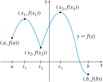
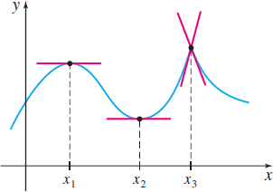
Figure 7 illustrates the graph of a function f defined on a closed interval [a,b]. Pay particular attention to the graph at the numbers x1, x2, and x3. In small open intervals containing x1 and x3 the value of f is greatest at these numbers. We say that f has local maxima at x1 and x3, and that f(x1) and f(x3) are local maximum values of f. Similarly, in small open intervals containing x2, the value of f is the least at x2. We say f has a local minimum at x2 and f(x2) is a local minimum value of f. (“Maxima” is the plural of “maximum”; “minima” is the plural of “minimum.”)
On the closed interval [a,b] , the largest value of f is f(x3), while the smallest value of f is f(b). These are called, respectively, the absolute maximum value and absolute minimum value of f on [a,b] .
264
DEFINITION Absolute Extrema
Let f be a function defined on an interval I. If there is a number u in the interval for which f(u)≥f(x) for all x in I, then f has an absolute maximum at u and the number f(u) is called the absolute maximum value of f on I.
If there is a number v in I for which f(v)≤f(x) for all x in I, then f has an absolute minimum at v and the number f(v) is the absolute minimum value of f on I.
The values f(u) and f(v) are sometimes called absolute extrema or the extreme values of f on I. (“Extrema” is the plural of the Latin noun extremum.)
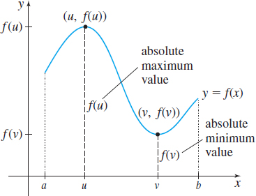
The absolute maximum value and the absolute minimum value, if they exist, are the largest and smallest values, respectively, of a function f on the interval I. See Figure 8. Contrast this idea with that of a local maximum value and a local minimum value. These are the largest and smallest values of f in some open interval in I. The next definition makes this distinction precise.
DEFINITION Local Extrema
Let f be a function defined on some interval I and let u and v be numbers in I. If there is an open interval in I containing u so that f(u)≥f(x) for all x in this open interval, then f has a local maximum (or relative maximum) at u, and the number f(u) is called a local maximum value.
Similarly, if there is an open interval in I containing v so that f(v)≤f(x) for all x in this open interval, then f has a local minimum (or a relative minimum) at v, and the number f(v) is called a local minimum value.
The term local extreme value describes either a local maximum value of f or a local minimum value of f.
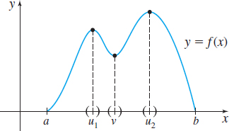
Figure 9 illustrates the definition.
Notice in the definition of a local maximum that the interval that contains u is required to be open. Notice also in the definition of a local maximum that the value f(u) must be greater than or equal to all other values of f in this open interval. The word “local” is used to emphasize that this condition holds on some open interval containing u. Similar remarks hold for a local minimum.
EXAMPLE 1Identifying Maximum and Minimum Values and Local Extreme Values from the Graph of a Function
Figures 10, 11, 12, 13, 14 and 15 show the graphs of six different functions. For each function:
NEED TO REVIEW?
Continuity is discussed in Section 1.3, pp. 93-102.
- (a) Find the domain.
- (b) Determine where the function is continuous.
- (c) Identify the absolute maximum value and the absolute minimum value, if they exist.
- (d) Identify any local extreme values.
Solution
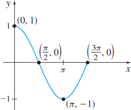
(b) Continuous on [0,3π2]
(c) Absolute maximum value:
f(0)=1
Absolute minimum value:
f(π)=−1
(d) No local maximum value;
local minimum value: f(π)=−1
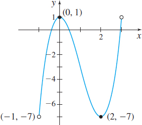
(b) Continuous on (−1,3)
(c) Absolute maximum value:
f(0)=1
Absolute minimum value:
f(2)=−7
(d) Local maximum value:
f(0)=1
Local minimum value:
f(2)=−7
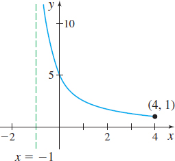
(b) Continuous on (−1,4]
(c) No absolute maximum value;
absolute minimum value:
f(4)=1
(d) No local maximum value;
no local minimum value
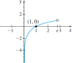
(b) Continuous on (0,e)
(c) No absolute maximum value;
no absolute minimum value
(d) No local maximum value;
no local minimum value
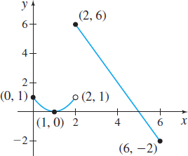
(b) Continuous on [0,6] except
at x=2
(c)Absolute maximum value:
f(2)=6
Absolute minimum value:
f(6)=−2
(d) Local maximum value: f(2)=6
Local minimum value: f(1)=0
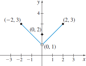
(b) Continuous on [−2,2] except at x=0
(c) Absolute maximum value:
f(−2)=3, f(2)=3
No absolute minimum value
(d) Local maximum value: f(0)=2
No local minimum value
265
NOW WORK
Example 1 illustrates that a function f can have both an absolute maximum value and an absolute minimum value, can have one but not the other, or can have neither an absolute maximum value nor an absolute minimum value. The next theorem provides conditions for which a function f will always have absolute extrema. Although the theorem seems simple, the proof requires advanced topics and may be found in most advanced calculus books.
THEOREM Extreme Value Theorem
If a function f is continuous on a closed interval [a,b], then f has an absolute maximum and an absolute minimum on [a,b].
Look back at Example 1. Figure 10 illustrates a function that is continuous on a closed interval; it has an absolute maximum and an absolute minimum on the interval. But if a function is not continuous on a closed interval [a,b], then the conclusion of the Extreme Value Theorem may or may not hold.
For example, the functions graphed in Figures 11, 12, and 13 are all continuous, but not on a closed interval:
- In Figure 11, the function has both an absolute maximum and an absolute minimum.
- In Figure 12, the function has an absolute minimum but no absolute maximum.
- In Figure 13, the function has neither an absolute maximum nor an absolute minimum.
266
On the other hand, the functions graphed in Figures 14 and 15 are each defined on a closed interval, but neither is continuous on that interval:
- In Figure 14, the function has an absolute maximum and an absolute minimum.
- In Figure 15, the function has an absolute maximum but no absolute minimum.
NOW WORK
The Extreme Value Theorem is an example of an existence theorem. It states that, if a function is continuous on a closed interval, then extreme values exist. It does not tell us how to find these extreme values. Although we can locate both absolute and local extrema given the graph of a function, we need tools that allow us to locate the extreme values analytically, when only the function f is known.
Consider the function y=f(x) whose graph is shown in Figure 16. There is a local maximum at x1 and a local minimum at x2. The derivative at these points is 0, since the tangent lines to the graph of f at x1 and x2 are horizontal. There is also a local maximum at x3, where the derivative fails to exist. The next theorem provides the details.
THEOREM Condition for a Local Maximum or a Local Minimum
If a function f has a local maximum or a local minimum at the number c, then either f′(c)=0 or f′(c) does not exist.
Proof
Suppose f has a local maximum at c. Then, by definition, f(c)≥f(x)
for all x in some open interval containing c. Equivalently, f(x)−f(c)≤0
The derivative of f at c may be written as f′(c)=lim
provided the limit exists. If this limit does not exist, then f^\prime (c) does not exist and there is nothing further to prove.
If this limit does exist, then \begin{equation*} \lim\limits_{x\rightarrow c^{-}}\frac{f(x)-f(c)}{x-c}={\lim\limits_{x \rightarrow c^{+}}}\frac{f(x)-f(c)}{x-c} \tag{1} \end{equation*}
In the limit on the left, x<c and f(x)-f(c)\leq 0, so \dfrac{f(x)-f(c)}{ x-c}\geq 0 and \begin{equation*} \lim\limits_{x\rightarrow c^{-}}\dfrac{f(x)-f(c)}{x-c}\geq 0 \tag{2} \end{equation*}
[Do you see why? If the limit were negative, then there would be an open interval about c, x<c, on which f(x) -f( c) <0; refer to Section 1.6, Example 7, p. 136.]
ORIGINS
Pierre de Fermat (1601–1665), a lawyer whose contributions to mathematics were made in his spare time, ranks as one of the great “amateur” mathematicians. Although Fermat is often remembered for his famous “last theorem,” he established many fundamental results in number theory and, with Pascal, cofounded the theory of probability. Since his work on calculus was the best done before Newton and Leibniz, he must be considered one of the principal founders of calculus.
Similarly, in the on the right side of (1), x>c and f(x)-f(c)\leq 0, so \dfrac{f(x)-f(c)}{x-c}\leq 0 and \begin{equation*} \lim\limits_{x\rightarrow c^{+}}\frac{f(x)-f(c)}{x-c}\leq 0 \tag{3} \end{equation*}
Since the limits (2) and (3) must be equal, we have {f}^{\prime }(c)=\lim\limits_{x\rightarrow c}\frac{f(x)-f(c)}{x-c}=0
The proof when f has a local minimum at c is similar and is left as an exercise (Problem 92).
267
For differentiable functions, the following theorem, often called Fermat’s Theorem, is simpler.
THEOREM
If a differentiable function f has a local maximum or a local minimum at c, then f^\prime ( c) =0.
In other words, for differentiable functions, local extreme values occur at points where the tangent line to the graph of f is horizontal.
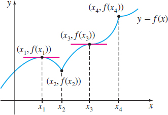
As the theorems show, the numbers at which a function f^\prime (x) =0 or at which f^\prime does not exist provide a clue for locating where f has local extrema. But unfortunately, knowing that f^\prime ( c) =0 or that f^\prime does not exist at c does not guarantee a local extremum occurs at c. For example, in Figure 17, f^\prime (x_{3})=0, but f has neither a local maximum nor a local minimum at x_{3}. Similarly, f^\prime (x_{4}) does not exist, but f has neither a local maximum nor a local minimum at x_{4}.
Even though there may be no local extrema found at the numbers c for which f^\prime (c)\,=\,0 or f^\prime ( c) do not exist, the collection of all such numbers provides all the possibilities where f might have local extreme values. For this reason, we call these numbers critical numbers.
DEFINITION Critical Number
A critical number of a function f is a number c in the domain of f for which either f^\prime ( c) =0 or f^\prime ( c) does not exist.
2 Find Critical NumbersPrinted Page 267
EXAMPLE 2Finding Critical Numbers
Find any critical numbers of the following functions:
- (a) f(x)=x^{3}-6x^{2}+9x+2
- (b) R(x)=\dfrac{1}{x-2}
- (c) g(x)=\dfrac{(x-2)^{2/3}}{x}
- (d) G(x)={\sin }\,x
Solution (a) Since f is a polynomial, it is differentiable at every real number. So, the critical numbers occur where f^\prime (x) =0. f^\prime (x) ={3x}^{2}-12x+9=3({x-1})({x-3})
f^\prime (x)=0 at x=1 and x=3; the numbers 1 and 3 are the critical numbers of f.
(b) The domain of R(x) = \dfrac{1}{x-2} is \{ x\,|\,x\neq 2\} , and R^\prime (x)=-\dfrac{\,1}{( x-2) ^{2} }. \ R^\prime exists for all numbers x in the domain of R (remember, 2 is not in the domain of R). Since R^\prime is never 0, R has no critical numbers.
(c) The domain of g(x)=\dfrac{(x\,{-}\,2)^{2/3}}{x} is \{ x\,|\,x\neq 0\} , and the derivative of g is \begin{eqnarray*} {{g^\prime }(x)}={\frac{x\cdot \left[ {\dfrac{2}{3}}({x-2})^{-1/3}\right] -1\cdot ({x-2})^{2/3}}{x^{2}}} \underset{\underset{{\color{#0066A7}{\hbox{Multiply by} \dfrac{3(x-2) ^{1/3}}{3( x-2) ^{1/3}}}}}{\color{#0066A7}{\uparrow}}}{=} {\frac{2x-3({x-2})}{3x^{2}({x-2})^{1/3}}=\frac{6-x}{3x^{2}({x-2})^{1/3}}}\\ \end{eqnarray*}
268
Critical numbers occur where g^\prime (x) =0 or where g^\prime (x) does not exist. If x=6, then g^\prime (6) =0. Next, g^\prime (x) does not exist where \begin{eqnarray*} \begin{array}{rl@{\qquad}r@{\qquad}rr} 3x^{2}( x-2) ^{1/3} &= 0 \\ 3x^{2} &= 0 & \hbox{ or } & ( x-2) ^{1/3} &= 0 \\ x &= 0 & \hbox{ or } & x &= 2 \end{array} \end{eqnarray*}
We ignore 0 since it is not in the domain of g. The critical numbers of g are 6 and 2.
(d) The domain of G is all real numbers. The function G is differentiable on its domain, so the critical numbers occur where G^\prime (x) =0. G^\prime (x)=\cos \,x and \cos x=0 at x=\pm \dfrac{\pi }{2}, {\pm }\dfrac{3\pi }{2}, {\pm }\dfrac{5\pi }{2},\ldots. This function has infinitely many critical numbers.
NOW WORK
We are not yet ready to give a procedure for determining whether a function f has a local maximum, a local minimum, or neither at a critical number. This requires the Mean Value Theorem, which is the subject of the next section. However, the critical numbers do help us find the extreme values of a function f.
3 Find Absolute Maximum and Absolute Minimum ValuesPrinted Page 268
The following theorem provides a way to find the extreme values of a function f that is continuous on a closed interval [ a,b] .
THEOREM Locating Extreme Values
Let f be a function that is continuous on a closed interval [a,b]. Then the absolute maximum value and the absolute minimum value of f are the largest and the smallest values, respectively, found among the following:
- The values of f at the critical numbers in the open interval (a,b)
- f(a) and f(b), the values of f at the endpoints a and b
For any function f satisfying the conditions of this theorem, the Extreme Value Theorem reveals that extreme values exist, and this theorem tells us how to find them.
Steps for Finding the Absolute Extreme Values of a Function f That Is Continuous on a Closed Interval {[ a,b]}
Step 1 Locate all critical numbers in the open interval ( a,b) .
Step 2 Evaluate f at each critical number and at the endpoints a and b.
Step 3 The largest value is the absolute maximum value; the smallest value is the absolute minimum value.
EXAMPLE 3Finding Absolute Maximum and Minimum Values
Find the absolute maximum value and the absolute minimum value of each function:
- (a) f(x)=x^{3}-6x^{2}+9x+2 on [0,2]
- (b) g(x)= \dfrac{(x-2)^{2/3}}{x} on [1,10]
Solution (a) The function f, a polynomial function, is continuous on the closed interval [0,2], so the Extreme Value Theorem guarantees that f has an absolute maximum value and an absolute minimum value on the interval. We follow the steps for finding the absolute extreme values to identify them.
Step 1 From Example 2(a), the critical numbers of f are 1 and 3. We exclude 3, since it is not in the interval (0,2) .
Step 2 Find the value of f at the critical number 1 and at the endpoints 0 and 2: f(1)=6\qquad f( 0) =2\qquad f(2) =4
Step 3 The largest value 6 is the absolute maximum value of f; the smallest value 2 is the absolute minimum value of f.
269
(b) The function g is continuous on the closed interval [1,10], so g has an absolute maximum and an absolute minimum on the interval.
Step 1 From Example 2(c), the critical numbers of g are 2 and 6. Both critical numbers are in the interval (1,10).
Step 2 We evaluate g at the critical numbers 2 and 6 and at the endpoints 1 and 10:
| x | {\dfrac{( x-2) ^{2/3}}{x}} | {g(x)} | |
|---|---|---|---|
| 1 | \dfrac{(1-2) ^{2/3}}{1}=(-1) ^{2/3} | 1 | \longleftarrow absolute maximum value |
| 2 | \dfrac{( 2-2) ^{2/3}}{2} | 0 | \longleftarrow absolute minimum value |
| 6 | \dfrac{(6-2) ^{2/3}}{6}=\dfrac{4^{2/3}}{6} | \approx\! 0.42 | |
| 10 | \dfrac{(10-2) ^{2/3}}{10}=\dfrac{8^{2/3}}{10}=\dfrac{4}{10} | 0.4 |
Step 3 The largest value 1 is the absolute maximum value; the smallest value 0 is the absolute minimum value.
NOW WORK
For piecewise-defined functions f, we need to look carefully at the number(s) where the rules for the function change.

EXAMPLE 4Finding Absolute Maximum and Minimum Values
Find the absolute maximum value and absolute minimum value of the function f(x)=\left\{ {{ \begin{array}{@{}l@{\qquad}l@{\quad}l} {2x-1} & \text{if} & {0\leq x\leq 2} \\ {x^{2}-5x+9} & \text{if} & {2<x\leq 3} \end{array} }}\right.
Solution The function f is continuous on the closed interval [0,3]. (You should verify this.) To find the absolute maximum value and absolute minimum value, we follow the three-step procedure.
Step 1 Find the critical numbers in the open interval (0,3):
- On the open interval (0, 2): f(x)= 2x-1 and f^\prime (x) =2. Since f^\prime (x) \neq 0 on the interval (0, 2) , there are no critical numbers in (0, 2).
- On the open interval (2, 3): f(x)=x^{2}-5x+9 and f^\prime (x) =2x - 5. Solving f^\prime (x) =2x-5=0, we find x=\dfrac{5}{2}. Since \dfrac{5}{2} is in the interval (2, 3), \dfrac{5}{2} is a critical number.
- At x=2, the rule for f changes, so we investigate the one-sided limits of \dfrac{f(x) -f(2) }{x-2}. \begin{eqnarray*} \lim\limits_{x\rightarrow 2^{-}}\dfrac{f(x) -f(2) }{ x-2} &=& \lim\limits_{x\rightarrow 2^{-}}\dfrac{(2x-1) -3}{x-2} =\lim\limits_{x\rightarrow 2^{-}}\dfrac{2x-4}{x-2}\\[3pt] &=&\lim\limits_{x\rightarrow 2^{-}}\dfrac{2(x-2) }{x-2}=2 \\[3pt] \lim\limits_{x\rightarrow 2^{+}}\dfrac{f(x) -f(2) }{ x-2} &=& \lim\limits_{x\rightarrow 2^{+}}\dfrac{(x^{2}-5x+9) -3}{x-2} =\lim\limits_{x\rightarrow 2^{+}}\dfrac{x^{2}-5x+6}{x-2}\\[3pt] &=&\lim\limits_{x \rightarrow 2^{+}}\dfrac{( x-2) (x-3) }{x-2} =\lim\limits_{x\rightarrow 2^{+}}(x-3) =-1 \end{eqnarray*}
270
The one-sided limits are not equal, so the derivative does not exist at 2; 2 is a critical number.
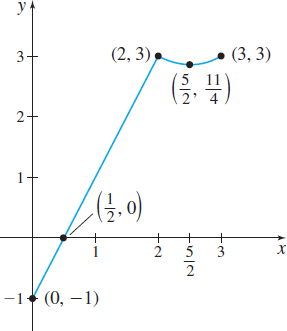
Step 2 Evaluate f at the critical numbers \dfrac{5}{2} and 2 and at the endpoints 0 and 3.
| x | {f(x)} | {f(x)} | |
|---|---|---|---|
| 0 | 2\cdot 0-1 | -1 | \longleftarrow absolute minimum value |
| 2 | 2\cdot 2-1 | 3 | \longleftarrow absolute maximum value |
| \dfrac{5}{2} | \left( \dfrac{5}{2}\right) ^{\!\!2}-5\left( \dfrac{5}{2}\right) +9=\dfrac{25}{4}-\dfrac{25}{2}+9 | \dfrac{11}{4} | |
| 3 | 3^{2}-5\cdot 3+9=9-15+9 | 3 | \longleftarrow absolute maximum value |
Step 3 The largest value 3 is the absolute maximum value; the smallest value -1 is the absolute minimum value.
The graph of f is shown in Figure 18. Notice that the absolute maximum occurs at 2 and at 3.
NOW WORK
EXAMPLE 5Constructing a Rain Gutter
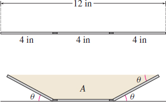
A rain gutter is to be constructed using a piece of aluminum 12 in wide. After marking a length of 4 \,{\rm in}. from each edge, the piece of aluminum is bent up at an angle \theta, as illustrated in Figure 19. The area A of a cross section of the opening, expressed as a function of \theta , is A(\theta) =16~\sin ~\theta ( \cos \theta +1)\qquad 0 \leq \theta \leq \dfrac{\pi }{2}
Find the angle \theta that maximizes the area A. (This bend will allow the most water to flow through the gutter.)
Solution The function A=A(\theta ) is continuous on the closed interval \left[ 0,\dfrac{\pi }{2}\right] . To find the angle \theta that maximizes A, we follow the three-step procedure.
Step 1 We locate all critical numbers in the open interval \left( 0,\dfrac{\pi }{2}\right). \begin{eqnarray*} A^\prime (\theta ) &=& 16\sin \theta (-\!\sin \theta) +16\cos \theta ( \cos \theta +1) \hspace{12pc} \color{#0066A7}{{\hbox{Product Rule}}}\\[3pt] &=& 16[-\!\sin ^{2}\theta +\cos^{2}\theta +\cos \theta] \\[3pt] &=& 16[ ( \cos ^{2}\theta -1) +\cos ^{2}\theta +\cos \theta ] \hspace{15pc} \color{#0066A7}{{\hbox{$\kern-.5pt-\!\sin^2\theta=\cos^2\theta-1$}}}\\[3pt] &=& 16[2\cos^{2}\theta +\cos \theta -1] = 16(2\cos \theta -1) (\cos \theta +1) \end{eqnarray*}
The critical numbers satisfy the equation A^\prime (\theta ) =0, 0<\theta<\frac{\pi}{2}. \begin{eqnarray*} \begin{array}{rl@{ }l@{ }rl} 16(2\;\cos \theta -1) ( \cos \theta +1) &= 0 \\[3pt] 2\;\cos \theta -1 &= 0 & \quad\hbox{ or }\quad & \cos \theta +1 &=0 \\[3pt] \cos \theta &= \dfrac{1}{2} & \hbox{ }& \cos \theta &=-1\\[3pt] \theta &= \dfrac{\pi }{3} \;{\rm or}\; \dfrac{5\pi }{3} & \hbox{ }& \theta &= \pi \end{array} \end{eqnarray*}
Of these solutions, only \dfrac{\pi }{3} is in the interval \left( 0,\dfrac{\pi }{2}\right). So, \dfrac{\pi }{3} is the only critical number.
271
Step 2 We evaluate A at the critical number \dfrac{\pi }{3} and at the endpoints 0 and \dfrac{\pi }{2}.
| \theta | {16\sin \theta ( \cos \theta +1)} | A(\theta ) | |
|---|---|---|---|
| 0 | 16\sin 0\left( \cos 0+1\right) =0 | 0 | |
| \dfrac{\pi }{3} | \begin{eqnarray*} 16&\sin \dfrac{\pi }{3}\left( \cos \dfrac{\pi }{3} +1\right) \\ &= 16\left(\dfrac{\sqrt{3}}{2}\right) \left(\dfrac{1}{2}+1\right) \\ &= 16\left( \dfrac{3\sqrt{3}}{4}\right) =12\sqrt{3} \end{eqnarray*} | \approx\!20.8 | \longleftarrow absolute maximum value |
| \dfrac{\pi }{2} | \begin{eqnarray*} 16&\sin \dfrac{\pi }{2}\left(\cos \dfrac{\pi }{2}+1\right) \\ &=16( 1) (0+1) =16 \end{eqnarray*} | 16 |
Step 3 If the aluminum is bent at an angle of \dfrac{\pi }{3}, the area of the opening is maximum. The maximum area is about 20.8 \,{\rm in}^{2}.
NOW WORK
From physics, the volume V of fluid flowing through a pipe is related to the radius r of the pipe and the difference in pressure p at each end of the pipe. It is given by the equation V=kpr^{4}
where k is a constant.
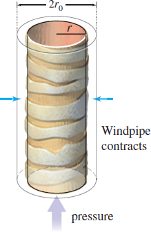
EXAMPLE 6Analyzing a Cough
Coughing is caused by increased pressure in the lungs and is accompanied by a decrease in the diameter of the windpipe. See Figure 20. The radius r of the windpipe decreases with increased pressure p according to the formula r_{0}-r=cp, where r_{0} is the radius of the windpipe when there is no difference in pressure and c is a positive constant. The volume V of air flowing through the windpipe is V=kpr^{4}
where k is a constant. Find the radius r that allows the most air to flow through the windpipe. Restrict r so that 0<\dfrac{r_{0}}{2}\leq r\leq r_{0}.
Solution
Since p= \dfrac{r_{0}-r}{c}, we can express V as a function of r: V=V(r) =k\!\left( \dfrac{r_{0}-r}{c}\right) r^{4}=\dfrac{k r_{0}}{c} r^{4}-\dfrac{k}{c} r^{5} \qquad \dfrac{r_{0}}{2}\leq r\leq r_{0}
Now we find the absolute maximum of V on the interval \left[\dfrac{r_{0}}{2},r_{0}\right]. V^\prime (r) =\dfrac{4k\,r_{0}}{c}\,r^{3}-\dfrac{5k}{c}\,r^{4}=\dfrac{k}{c}\,r^{3}(4r_{0}-5r)
The only critical number in the interval \left( \dfrac{r_{0}}{2}, r_{0}\right) is r=\dfrac{4r_{0}}{5}.
272
We evaluate V at the critical number and at the endpoints, \dfrac{r_{0}}{2} and r_{0}.
| {r} | {V(r) =k\left( \dfrac{r_{0}-r}{c}\right) r^{4}} |
|---|---|
| \dfrac{r_{0}}{2} | k\left( \dfrac{r_{0}-\dfrac{r_{0}}{2}}{c}\right) \left( \dfrac{r_{0}}{2}\right) ^{\!\!4}=\dfrac{k\,r_{0}^{5}}{32c} |
| \dfrac{4r_{0}}{5} | k\left( \dfrac{r_{0}-\dfrac{4r_{0}}{5}}{c}\right) \left( \dfrac{4r_{0}}{5}\right) ^{\!\!4}=\dfrac{k}{c}\cdot \dfrac{ 4^{4}\,r_{0}^{5}}{5^{5}}=\dfrac{256\,k\,r_{0}^{5}}{3125c} |
| r_{0} | 0 |
The largest of these three values is \dfrac{256\,kr_{0}^{5}}{3125c}. So, the maximum air flow occurs when the radius of the windpipe is \dfrac{4r_{0}}{5}, that is, when the windpipe contracts by 20\%.