4.3 The Mean Value TheoremPrinted Page 275
OBJECTIVES
When you finish this section, you should be able to:
ORIGINS
Michel Rolle (1652–1719) was a French mathematician whose formal education was limited to elementary school. At age 24, he moved to Paris and married. To support his family, Rolle worked as an accountant, but he also began to study algebra and became interested in the theory of equations. Although Rolle is primarily remembered for the theorem proved here, he was also the first to use the notation n√ for the nth root.
In this section, we prove several theorems. The most significant of these, the Mean Value Theorem, is used to develop tests for locating local extreme values. To prove the Mean Value Theorem, we need Rolle’s Theorem.
1 Use Rolle’s TheoremPrinted Page 275
THEOREM Rolle’s Theorem
Let f be a function defined on a closed interval [a,b]. If:
- f is continuous on [a,b],
- f is differentiable on (a,b), and
- f(a)=f(b),
then there is at least one number c in the open interval (a,b) for which f′(c)=0.
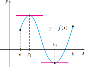
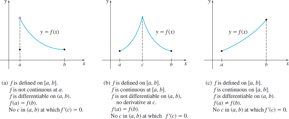
Before we prove Rolle’s Theorem, notice that the graph in Figure 21 meets the three conditions of Rolle’s Theorem and has at least one number c at which f′(c)=0.
In contrast, the graphs in Figure 22 show that the conclusion of Rolle’s Theorem may not hold when one or more of the three conditions are not met.
276
Proof
Because f is continuous on a closed interval [a,b], the Extreme Value Theorem guarantees that f has an absolute maximum value and an absolute minimum value on [a,b] . There are two possibilities:
- If f is a constant function on [a,b], then f′(x)=0 for all x in (a,b).
- If f is not a constant function on [a,b], then, because f(a)=f(b), either the absolute maximum or the absolute minimum occurs at some number c in the open interval (a,b). Then f(c) is a local maximum value (or a local minimum value), and, since f is differentiable on (a,b), f′(c)=0.
EXAMPLE 1Using Rolle’s Theorem
Find the x-intercepts of f(x)=x2−5x+6, and show that f′(c)=0 for some number c belonging to the interval formed by the two x-intercepts. Find c.
Solution At the x-intercepts, f(x)=0. f(x)=x2−5x+6=(x−2)(x−3)=0
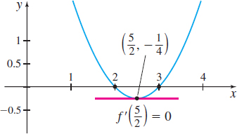
So, x=2 and x=3 are the x-intercepts of the graph of f, and f(2)= f(3)=0.
Since f is a polynomial, it is continuous on the closed interval [2,3] formed by the x-intercepts and is differentiable on the open interval (2,3). The three conditions of Rolle’s Theorem are satisfied, guaranteeing that there is a number c in the open interval (2,3) for which f′(c)=0. Since f′(x)=2x−5, the number c for which f′(x)=0 is c=52.
See Figure 23 for the graph of f.
NOW WORK
2 Work with the Mean Value TheoremPrinted Page 276
The real importance of Rolle’s Theorem is that it can be used to obtain other results, many of which have wide-ranging application. Perhaps the most important of these is the Mean Value Theorem, sometimes called the Theorem of the Mean for Derivatives.
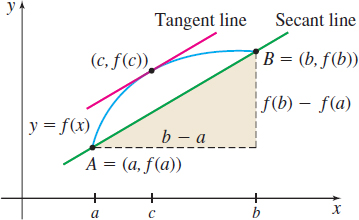


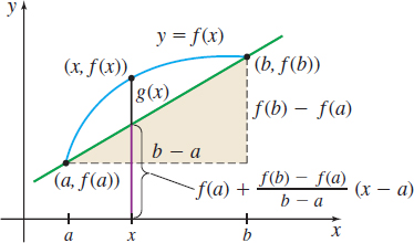
We can provide a geometric example to motivate the Mean Value Theorem. Consider the graph of a function f that is continuous on a closed interval [a,b] and differentiable on the open interval (a,b), as illustrated in Figure 24. Then there is at least one number c between a and b at which the slope f′(c) of the tangent line to the graph of f equals the slope of the secant line joining the points A=(a, f(a)) and B=(b, f(b)). That is, there is at least one number c in the open interval (a,b) for which f′(c)=f(b)−f(a)b−a
277
THEOREM Mean Value Theorem
Let f be a function defined on a closed interval [a,b]. If:
- f is continuous on [a,b]
- f is differentiable on (a,b),
then there is at least one number c in the open interval (a,b) for which \begin{equation*}{\bbox[#FAF8ED,5pt]{\bbox[5px, border:1px solid black, #F9F7ED]{ {f^\prime (c) =\dfrac{f(b) -f(a)}{b-a}}}}} \tag{1} \end{equation*}
Proof
We begin by finding the slope m_{\sec } of the secant line containing points (a, f(a)) and (b, f(b)). m_{\sec }=\dfrac{f(b) -f(a) }{b-a}
Then using the point (a,f(a)) and the point slope form of an equation of a line, an equation of this secant line is y-f(a) =\dfrac{f(b) -f(a) }{b-a}(x-a)
so y=f(a) +\dfrac{f(b) -f(a) }{b-a}(x-a)
NOTE
The function g has a geometric significance: Its value equals the vertical distance from the graph of y = f(x) to the secant line joining (a, \ \ f(a)) to (b, \ \ f(b)). See Figure 25.
Now we construct a function g that satisfies the conditions of Rolle’s Theorem, by defining g as g(x)=f(x)-\underset{\color{#0066A7}{\hbox{Height of the secant line}\atop \hbox{containing \((a,\;f(a))\) and \((b,\;f(b))\)} }}{\underbrace{\hbox{\(\left[ {f(a)+\frac{f(b)-f(a)}{b-a}({x-a})}\right]\)} }}
for all x on [ a,b].
Since f is continuous on [a,b] and differentiable on (a,b), it follows that g is also continuous on [a,b] and differentiable on (a,b). Also, \begin{array}{l} g\left( a \right) = f\left( a \right) - \left[ {f\left( a \right) + \frac{{f\left( b \right) - f\left( a \right)}}{{b - a}}\left( {a - a} \right)} \right] = 0 \\ g\left( b \right) = f\left( b \right) - \left[ {f\left( a \right) + \frac{{f\left( b \right) - f\left( a \right)}}{{b - a}}\left( {b - a} \right)} \right] = 0 \\ \end{array}
Now, since g satisfies the three conditions of Rolle’s Theorem, there is a number c in (a,b) at which g^\prime (c)=0. Since f(a) and \dfrac{f(b)-f(a)}{b-a} are constants, g^\prime (x) is given by g^\prime (x)=f^\prime (x)-\frac{f(b)-f(a)}{b-a}
Now we evaluate g^\prime at c and use the fact that g^\prime (c) = 0. \begin{array}{l} g'\left( c \right) = f'\left( c \right) - \left[ {\frac{{f\left( b \right) - f\left( a \right)}}{{b - a}}} \right] = 0 \\ f'\left( c \right) = \frac{{f\left( b \right) - f\left( a \right)}}{{b - a}} \\ \end{array}
The Mean Value Theorem is another example of an existence theorem. It does not tell us how to find the number c; it merely states that at least one number c exists. Often, the number c can be found.
278

EXAMPLE 2Verifying the Mean Value Theorem
Verify that the function f(x)=x^{3}-3x+5, -1\leq x\leq 1 satisfies the conditions of the Mean Value Theorem. Find the number(s) c guaranteed by the Mean Value Theorem.
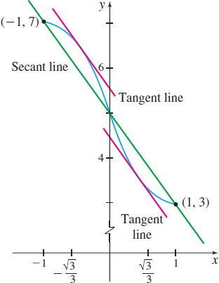
Solution Since f is a polynomial function, f is continuous on the closed interval [-1,1] and differentiable on the open interval (-1,1). The conditions of the Mean Value Theorem are met. Now, f(-1) =7\qquad f(1) =3\qquad \hbox{ and }\qquad f^\prime (x) =3x^{2}-3
The number(s) c in the open interval (-1,1) guaranteed by the Mean Value Theorem satisfy the equation \begin{array}{l} \ \ \ \ f'\left( c \right) = \frac{{f\left( 1 \right) - f\left( { - 1} \right)}}{{1 - \left( { - 1} \right)}} \\ 3{c^2} - 3 = \frac{{3 - 7}}{{1 - \left( { - 1} \right)}} = \frac{{ - 4}}{2} = - 2 \\ \ \ \ \ \ \ 3{c^2} = 1 \\ \ \ \ \ \ \ \ \ \ \ c = \sqrt {\frac{1}{3}} = \frac{{\sqrt 3 }}{3}\,\,\,\,\,\,{\rm{or}}\,\,\,\,\,\,\,c = - \sqrt {\frac{1}{3}} = - \frac{{\sqrt 3 }}{3} \\ \end{array}
There are two numbers in the interval (-1,1) that satisfy the Mean Value Theorem. See Figure 26.
NOW WORK
The Mean Value Theorem can be applied to rectilinear motion. Suppose the function s=f(t) models the distance s that an object has traveled from the origin at time t. If f is continuous on [a,b] and differentiable on (a,b), the Mean Value Theorem tells us that there is at least one time t at which the velocity of the object equals its average velocity.
Let t_{1} and t_{2} be two distinct times in [ a,b]. Then \begin{array}{l} {\rm{Average \ velocity \ over \ }}\left[ {{t_1},\,{t_2}} \right] = \frac{{f\left( {{t_2}} \right) - f\left( {{t_1}} \right)}}{{{t_2} - {t_1}}} \\ \,\,\,\,\,{\rm{Instantaneous \ velocity \ }}v \ \left( t \right) = \frac{{ds}}{{dt}} = f'\left( t \right) \\ \end{array}
The Mean Value Theorem states there is a time t_{0} in the interval (t_{1},t_{2}) for which f^\prime (t_{0})=\frac{f(t_{2})-f(t_{1})}{t_{2}-t_{1}}
That is, at time t_{0}, the velocity equals the average velocity over the interval [t_{1},t_{2}].
EXAMPLE 3Applying the Mean Value Theorem to Rectilinear Motion
Use the Mean Value Theorem to show that a car that travels 110 mi in 2 h must have had a speed of 55 miles per hour (mph) at least once during the 2 h.
Solution Let s= f(t) represent the distance s the car has traveled after t hours. Its average velocity during the time period from 0 to 2 h is \hbox{Average velocity}=\frac{f(2)-f(0)}{2-0}=\frac{110-0}{2-0}=55\ {\rm mph}
Using the Mean Value Theorem, there is a time t_{0}, 0<t_{0}<2, at which f^\prime (t_{0}) =\dfrac{f(2) -f( 0) }{2-0}=55
That is, the car had a velocity of 55 mph at least once during the 2 hour period.
NOW WORK
279
The following corollaries are a consequence of the Mean Value Theorem.
IN WORDS
If f^\prime ({x}) = 0 for all numbers in ({a,b}), then f is a constant function.
COROLLARY
If a function f is continuous on the closed interval [a, b] and is differentiable on the open interval ( a,b), and if f^\prime (x) =0 for all numbers x in ( a,b), then f is constant on (a,b).
Proof
To show that f is a constant function, we must show that f(x_{1}) =f(x_{2}) for any two numbers x_{1} and x_{2} in the interval (a,b).
Suppose x_{1}<x_{2}. The conditions of the Mean Value Theorem are satisfied on the interval [x_{1}, x_{2}], so there is a number c in this interval for which f^\prime ( c) =\dfrac{f( x_{2}) -f(x_{1}) }{x_{2}-x_{1}}
Since f^\prime ( c) =0 for all numbers in (a,b), we have \begin{array}{l} \,\,\,\,\,\,\,\,\,\,0 = \frac{{f\left( {{x_2}} \right) - f\left( {{x_1}} \right)}}{{{x_2} - {x_1}}} \\ \,\,\,\,\,\,\,\,\,\,0 = f\left( {{x_2}} \right) - f\left( {{x_1}} \right) \\ f\left( {{x_1}} \right) = f\left( {{x_2}} \right) \\ \end{array}
Applying the above corollary to rectilinear motion, if the velocity v of an object is zero over an interval (t_{1},t_{2}) , then the object does not move during this time interval.
IN WORDS
If two functions f and g have the same derivative, then the functions differ by a constant, and the graph of f is a vertical shift of the graph of g.
COROLLARY
If the functions f and g are differentiable on an open interval (a,b) and if f^\prime (x) =g^\prime (x) for all numbers x in (a,b), then there is a number C for which f(x) =g(x) +C on (a,b).
Proof
We define the function h so that h(x) =f(x) -g(x). Then h is differentiable since it is the difference of two differentiable functions, and h^\prime (x) =f^\prime (x) -g^\prime (x) =0
Since h^\prime (x) =0 for all numbers x in the interval ( a,b), h is a constant function and we can write h(x) =f(x) -g(x) =C \qquad \hbox{for some number }C
That is, f(x) =g(x) +C
3 Identify Where a Function Is Increasing and DecreasingPrinted Page 279
A third corollary that follows from the Mean Value Theorem gives us a way to determine where a function is increasing and where a function is decreasing. Recall that functions are increasing or decreasing on intervals, either open or closed or half-open or half-closed.
NEED TO REVIEW?
Increasing and decreasing functions are discussed in Section P.1, pp. 10-11.
COROLLARY Increasing/Decreasing Function Test
Let f be a function that is differentiable on the open interval (a,b):
- If f^\prime (x) >0 on ( a,b), then f is increasing on ( a,b).
- If f^\prime (x) <0 on ( a,b), then f is decreasing on ( a,b).
The proof of the first part of the corollary is given here. The proof of the second part is left for the exercises. See Problem 72.
280
Proof
Since f is differentiable on ( a,b), it is continuous on ( a,b). To show that f is increasing on ( a,b), we choose two numbers x_{1} and x_{2} in ( a,b), with x_{1}<x_{2}. We need to show that f(x_{1}) <f(x_{2}).
Since x_{1} and x_{2} are in ( a,b), f is continuous on the closed interval [x_{1},x_{2}] and differentiable on the open interval (x_{1}, x_{2}). By the Mean Value Theorem, there is a number c in the interval (x_{1}, x_{2}) for which f^\prime\left( c \right) = \frac{{f\left( {{x_2}} \right) - f\left( {{x_1}} \right)}}{{{x_2} - {x_1}}}
Since f^\prime (x) >0 for all x in (a, b), it follows that f^\prime\left( c \right) > 0. Since x_{1} < x_{2}, then x_{2}-x_{1}>0. As a result, \begin{array}{l} f\left( {{x_2}} \right) - f\left( {{x_1}} \right) > 0 \\ \,\,\,\,\,\,\,\,\,\,\,\,\,\,\,\,\,\,\,f\left( {{x_1}} \right) < f\left( {{x_2}} \right) \\ \end{array}
So, f is increasing on (a,b).
There are a few important observations to make about the Increasing/Decreasing Function Test:
- In using the Increasing/Decreasing Function Test, we determine open intervals on which the derivative is positive or negative.
Suppose f is continuous on the closed interval [a,b] and differentiable on the open interval ( a,b).
If f^\prime (x) >0 on (a,b), then f is increasing on the closed interval [ a,b].
If f^\prime (x) <0 on (a,b), then f is decreasing on the closed interval [ a,b].
- The Increasing/Decreasing Function Test is valid if the interval ( a,b) is ( -\infty ,b) or (a,\infty) or (-\infty, \infty).
NEED TO REVIEW?
Solving inequalities is discussed in Appendix A.1, pp. A-5 to A-8.
EXAMPLE 4Identifying Where a Function Is Increasing and Decreasing
Determine where the function f(x)=2x^{3}-9x^{2}+12x-5 is increasing and where it is decreasing.
Solution The function f is a polynomial so f is continuous and differentiable at every real number. We find f^\prime . f^\prime (x) =6x^{2}-18x+12=6({x-2})({x-1})
The Increasing/Decreasing Function Test states that f is increasing on intervals where f^\prime (x) >0 and that f is decreasing on intervals where f^\prime (x) <0. We solve these inequalities by using the numbers 1 and 2 to form three intervals, as shown in Figure 27. Then we determine the sign of f^\prime (x) on each interval, as shown in Table 1.
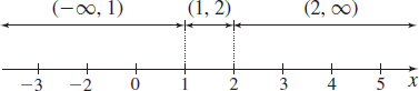
| Interval | Sign of {x-1} | Sign of {x-2} | Sign of f^\prime (x) = 6( x-2) ( x-1) | Conclusion |
|---|---|---|---|---|
| ( -\infty ,1) | Negative (-) | Negative (-) | Positive (+) | f is increasing |
| (1,2) | Positive (+) | Negative (-) | Negative (-) | f is decreasing |
| (2,\infty ) | Positive (+) | Positive (+) | Positive (+) | f is increasing |
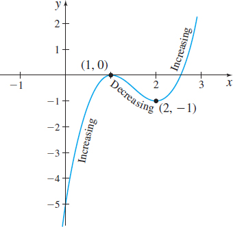
We conclude that f is increasing on the intervals (-\infty ,1) and (2,\infty), and f is decreasing on the interval (1,2).
The graph of f is shown in Figure 28. Notice that the graph of f has horizontal tangent lines at the points (1,0) and (2,-1). Also, since f is continuous on its domain, we can say that f is increasing on the intervals (-\infty ,1] and [2,\infty) and is decreasing on the interval [1,2].
281
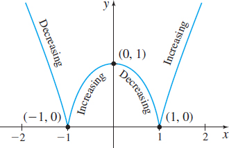
EXAMPLE 5Identifying Where a Function Is Increasing and Decreasing
Determine where the function f(x)=(x^{2}-1)^{2/3} is increasing and where it is decreasing.
Solution f is continuous for all numbers x, and f^\prime (x)=\frac{2}{3}({x^{2}-1})^{-1/3}({2x})=\frac{4x}{3({x^{2}-1})^{1/3}}
The Increasing/Decreasing Function Test states that f is increasing on intervals where f^\prime (x) >0 and decreasing on intervals where f^\prime (x) <0. We solve these inequalities by using the numbers -1, 0, and 1 to form four intervals. Then we determine the sign of f^\prime in each interval, as shown in Table 2. We conclude that f is increasing on the intervals (-1,0) and (1,\infty) and that f is decreasing on the intervals (-\infty ,-1) and (0,1).
| Interval | Sign of 4x | Sign of (x^{2}-1) ^{1/3} | Sign of f'\left( x \right) = \frac{{4x}}{{3{{\left( {{x^2} - 1} \right)}^{1/3}}}} | Conclusion |
|---|---|---|---|---|
| ( -\infty ,-1) | Negative (-) | Positive (+) | Negative (-) | f is decreasing on (-\infty,-1) |
| (-1,0) | Negative (-) | Negative (-) | Positive (+) | f is increasing on (-1,0) |
| (0,1) | Positive (+) | Negative (-) | Negative (-) | f is decreasing on (0,1) |
| (1,\infty) | Positive (+) | Positive (+) | Positive (+) | f is increasing on (1,\infty) |
Figure 29 shows the graph of f. Since f^\prime (0) =0, the graph of f has a horizontal tangent line at the point (0,1). Notice that f^\prime does not exist at \pm 1. Since f^\prime becomes unbounded at -1 and 1, the graph of f has vertical tangent lines at the points (-1,0) and (1,0). Also since f is continuous on its domain, we can say that f is increasing on the intervals [-1,0] and [1,\infty ) and is decreasing on the intervals (-\infty ,1] and [0,1].
NOW WORK
EXAMPLE 6Determining Crop Yield *
A variation of the von Liebig model states that the yield f(x) of a plant, measured in bushels, responds to the amount x of potassium in a fertilizer according to the following square root model: f(x) =-0.057-0.417x+0.852\sqrt{x}
For what amounts of potassium will the yield increase? For what amounts of potassium will the yield decrease?
Solution The yield is increasing when f^\prime (x)>0. f^\prime (x) =-0.417+\dfrac{0.426}{\sqrt{x}}=\dfrac{-0.417\sqrt{x}+0.426}{\sqrt{x}}
282
Now, f^\prime (x) >0 when \begin{array}{l} - 0.417\sqrt x + 0.426 > 0 \\ \,\,\,0.417\sqrt x - 0.426 < 0 \\ \,\,\,\,\,\,\,\,\,\,\,\,\,\,\,\,\,\,\,\,\,\,\,\,\,\,\,\,\,\,\,\,\,\,\,\sqrt x < 1.022 \\ \,\,\,\,\,\,\,\,\,\,\,\,\,\,\,\,\,\,\,\,\,\,\,\,\,\,\,\,\,\,\,\,\,\,\,\,\sqrt x < 1.044 \\ \end{array}
The crop yield is increasing when the amount of potassium in the fertilizer is less than 1.044 and is decreasing when the amount of potassium in the fertilizer is greater than 1.044.
*Source: Quirino Paris. (1992). The von Liebig Hypothesis. American Journal of Agricultural Economics, 74(4), 1019–1028.