14.2 The Double Integral over Nonrectangular RegionsPrinted Page 911
In the previous section, we used Fubini’s Theorem to find the double integral of a function \(f\) defined on a closed rectangular region. Although single integrals are always integrated over an interval, for double integrals the region of integration is not always rectangular. In this section, we see that Fubini’s Theorem extends to double integrals defined over certain closed, bounded regions, which we classify as \(x\)-simple and \(y\)-simple regions.
RECALL
A region \(R\) in the plane is closed if it contains all its boundary points. A region \(R\) is bounded if it can be enclosed by some circle, or equivalently, some rectangle in the plane.
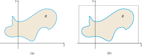
Suppose \(z=f(x,y) \) is a function of two variables defined on a closed, bounded region \(R\). See Figure 8(a) on page 912. Then \(R\) can be enclosed in a rectangle, as shown in Figure 8(b).
We partition the rectangle into subrectangles by drawing lines parallel to the coordinate axes, as shown in Figure 9(a). Then we discard all subrectangles that do not lie entirely in \(R\), as shown in Figure 9(b).
912
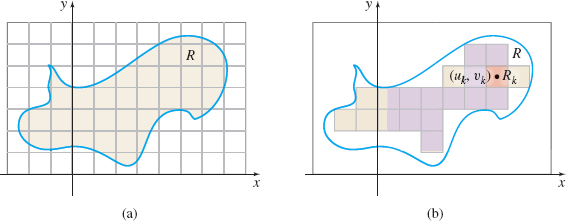
After doing this, suppose \(R_k,k=1,2,\ldots,N\), subrectangles remain. Choose a point \((u_{k},v_{k}) \) in each of the remaining \(N\) subrectangles and evaluate \( f(u_{k},v_{k})\). If \(\Delta A_{k}\) is the area of the \(k^{\it th}\) subrectangle, \(k=1,2,3,\ldots ,N\), we can form the Riemann sums \( \sum\limits_{k=1}^{N}f(u_{k},v_{k}) \Delta A_{k}.\) We define the norm \(\left\Vert P\right\Vert \) to be the longest diagonal of the subrectangles \(R_{k}\), \(k=1,2,\ldots ,N\). The double integral of the function \(z=f(x,y) \) defined on the closed, bounded region \(R\) is \[\bbox[5px, border:1px solid black, #F9F7ED]{ \displaystyle\iint\limits_{\kern-3ptR}f(x,y)\,{\it dA}=\lim\limits_{\Vert P\Vert \rightarrow 0}\sum\limits_{k=1}^{N}f(u_{k},v_{k}) \Delta A_{k} } \]
provided the limit exists.
A condition under which \(\lim\limits_{\Vert P\Vert \rightarrow 0}\sum\limits_{k=1}^{N}f(u_{k},v_{k}) \Delta A_{k}\) exists is given next. It extends the result given in Section 14.1 to regions that are not necessarily rectangular.
THEOREM Existence of a Double Integral
If a function \(z=f(x,y)\) is continuous on a closed, bounded region \(R\), then \(\iint\limits_{\kern-3ptR}f(x,y)\, {\it dA}\) exists.
When \(\iint\limits_{\kern-3ptR}f(x,y)\, {\it dA}\) exists, we say \(f\) is integrable on \(R\).
If \(z=f(x,y) \geq 0\) on a closed, bounded region \(R,\) then the double integral \(\iint\limits_{\kern-3ptR}f(x,y) \, {\it dA}\) equals the volume of the solid under the surface \(z=f(x,y) \) and over the region \( R \).
To see why, we partition \(R\), as before, into subrectangles by drawing lines parallel to the coordinate axes and discarding all subrectangles that do not lie entirely in \(R.\) Suppose \(N\) subrectangles remain. Figure 10 shows a typical subrectangle \(R_{k}\) that results from partitioning \(R\). We denote its area by \(\Delta A_{k},\) \(k=1,2,3,\ldots ,N.\)
913
Now suppose \(z=f(x,y)\) is a function of two variables that is continuous and nonnegative on the closed, bounded region \(R\). Then \(z\) is a surface lying above the \(xy\)-plane. Pick a point \((u_{k},v_{k}) \) in \(R_{k}\). The value \(f(u_{k},v_{k}) \) is the height of a rectangular solid whose base has the area \(\Delta A_{k}\). The volume \(V_{k}\) of this subrectangular solid is \(V_{k}=f(u_{k},v_{k}) \Delta A_{k}\). The sums \(\sum\limits_{k=1}^{N}f(u_{k},v_{k}) \Delta A_{k}\) over all the subrectangles of the partition approximate the volume \(V\) of the solid under the graph of the surface \(z=f(x,y)\) and above \(R\). But the sums are also an approximation to the double integral \(\displaystyle\iint\limits_{\kern-3ptR} f(x,y)\,dA\). As a result, the double integral \(\displaystyle\iint\limits_{\kern-3ptR} f(x,y)\,dA\) equals the volume of the solid under the surface \(z=f(x,y) \) and over the region \(R.\)

Volume Under a Surface and over a Region \(R\)
Let \(z=f(x,y) \) be a function of two variables that is continuous and nonnegative on a closed, bounded region \(R\). The volume \(V\) under the surface \(z=f(x,y)\) and over the region \(R\) is given by the double integral \[\bbox[5px, border:1px solid black, #F9F7ED]{ V=\displaystyle\iint\limits_{\kern-3ptR} f(x,y)\,dA } \]
Certain types of regions have properties that make it possible to find double integrals. One such type of region is called \(x\)-simple.
DEFINITION \(x\)-Simple Region
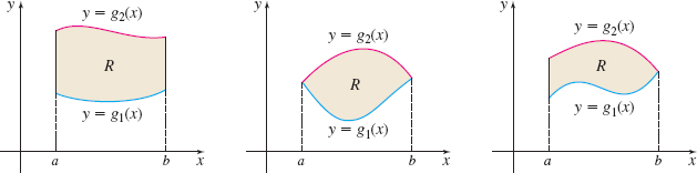
Let \(R\) be a closed, bounded region. \(R\) is an x-simple region if the boundary of \(R\) consists of two smooth curves, \(y=g_{1}(x)\) and \(y=g_{2}(x),\) each defined on a closed interval \([a,b] \), where \(g_{1}(x)\leq g_{2}(x)\) on \([a,b] .\) The boundary may also consist of a portion of the vertical lines \(x=a\) and \(x=b.\)
NEED TO REVIEW?
Smooth curves are discussed in Section 11.2, p. 768.
Figure 11 illustrates some typical \(x\)-simple regions. Notice in each case that the top and bottom boundaries of \(R\) can be expressed as functions of \( x,\) as the name \(x\)-simple implies.
Fubini’s Theorem can be extended to regions that are \(x\)-simple.
THEOREM Fubini’s Theorem for an \(x\)-Simple Region
If a function \(z=f(x,y) \) of two variables is continuous on a closed, bounded region \(R\) that is \(x\)-simple, then the double integral of \(f\) on \(R\) is given by \[\bbox[5px, border:1px solid black, #F9F7ED]{ \displaystyle\iint\limits_{\kern-3ptR}(x,y)\,dA=\int_{a}^{b} \left[ \int_{g_{1}(x)}^{g_{2}(x)}f(x,y)\,dy\right] dx } \]
where \(y=g_{1}(x)\) and \(y=g_{2}(x)\), \(g_{1}(x) \leq g_{2}(x)\), \(a \leq x \leq b\), are two smooth curves that form the boundary of \(R\).
914
The proof of Fubini’s Theorem can be found in advanced calculus books. Here, we give a geometric argument for Fubini’s Theorem for \(x\)-simple regions when \(f(x,y)\geq 0\) is continuous on \(R\).
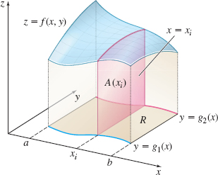
Suppose we choose a number \(x_{i}\) in the closed interval \([a,b]\) and let \( A(x_{i})\) equal the area of the intersection of the plane \(x=x_{i}\) and the solid under the surface \(z=f(x,y)\) and over \(R.\) See Figure 12. Using the slicing method, the volume \(V\) of the solid under \(z=f(x,y)\) and over \(R\) from \(x=a\) to \(x=b\) is given by \[ V=\int_{a}^{b}A(x)\,dx \]
Since this volume \(V\) is also given by \(V=\iint\limits_{\kern-3ptR} f(x,y)\,dA,\) we have \[ \begin{equation} V=\displaystyle\iint\limits_{\kern-3ptR} f(x,y)\,dA=\int_{a}^{b}A(x)\,dx\tag {1} \end{equation} \]
But \(A(x_{i})\) is the area of the plane region under the surface \( z=f(x_{i},y)\) from \(y=g_{1}(x_{i})\) to \(y=g_{2}(x_{i})\). That is, \begin{equation*} A(x)=\int_{g_{1}(x)}^{g_{2}(x)}f(x,y)\,dy \end{equation*}
NEED TO REVIEW?
Finding the volume of a solid using the slicing method is discussed in Section 6.4, pp. 433-437.
where \(x\) is held constant. By substituting \( \int_{g_{1}(x)}^{g_{2}(x)}f(x,y)\,{\it dy}\) for \(A(x)\) in the volume formula (1), we find \[ V=\displaystyle\iint\limits_{\kern-3ptR} f(x,y)\,dA=\int_{a}^{b}\underset{\color {#0066A7}{\hbox{\(A(x)\)}}}{ \underbrace{\left[ \int_{g_{1}(x)}^{g_{2}(x)}f(x,y)\,dy\right] }}dx \]
1 Use Fubini’s Theorem for an \(x\)-Simple RegionPrinted Page 914
EXAMPLE 1Use Fubini’s Theorem for an \(x\)-Simple Region
Find \(\iint\limits_{\kern-3ptR} xy\,dA\) if \(R\) is the region enclosed by \(y=x^{2}\) and \(y=\sqrt{x}.\)
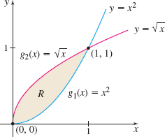
Solution We begin by graphing the region \(R.\) See Figure 13. Observe that \(R\) is a closed, bounded region. Also notice that the bottom and top boundaries of \(R\) are smooth curves expressed as functions of \(x\): \(g_{1}(x) =x^{2}\), \(g_{2}(x)=\sqrt{x}\), \(0\leq x\leq 1\). That is, \(R\) is \(x\)-simple, so we can use Fubini’s Theorem. \begin{eqnarray*} \displaystyle\iint\limits_{\kern-3ptR} xy\,{\it dA} &=&\int_{0}^{1}\left[ \int_{x^{2}}^{\sqrt{x}}xy\,{\it dy} \right] \! {\it dx}=\int_{0}^{1}x \left[ \dfrac{y^{2}}{2}\right] _{x^{2}}^{ \sqrt{x}}{\it dx}\\[4pt] &=&\int_{0}^{1}x\!\left(\dfrac{x-x^{4}}{2}\right)\!{\it dx}=\dfrac{1}{2} \int_{0}^{1}(x^{2}-x^{5})\,{\it dx}\\[4pt] &=&\dfrac{1}{2}\left[ \dfrac{x^{3}}{3}-\dfrac{x^{6}}{6}\right] _{0}^{1}=\dfrac{1 }{12} \end{eqnarray*}
NOW WORK
Regions whose left and right boundaries consist of smooth curves expressed as functions of \(y\) are referred to as \(y\)-simple regions.
915
DEFINITION \(y\)-Simple Region
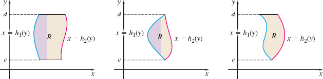
Let \(R\) be a closed, bounded region. Then \(R\) is a \(y\)-simple region if the boundary of \(R\) consists of two smooth curves, \(x=h_{1}(y)\) and \(x=h_{2}(y),\) each defined on the closed interval \(c\leq y\leq d,\) where \(h_{1}(y)\leq h_{2}(y)\) on \(\left[ c,d\right] .\) The boundary may also consist of a portion of the horizontal lines \(y=c\) and \(y=d\).
Figure 14 illustrates some typical \(y\)-simple regions.
Fubini’s Theorem also applies to closed, bounded regions that are \(y\)-simple.
THEOREM Fubini’s Theorem for an \(y\)-Simple Region
If a function \(f\) of two variables is continuous on a closed, bounded region \(R\) that is \(y\)-simple, the double integral of \(f\) on \(R\) is given by \[\bbox[5px, border:1px solid black, #F9F7ED]{ \displaystyle\iint\limits_{\kern-3ptR} f(x,y)\,dA=\int_{c}^{d}\left[ \int_{h_{1}(y)}^{h_{2}(y)}f(x,y)\,{\it dx}\right] dy } \]
where \(x=h_{1}(y)\) and \(x=h_{2}(y)\), \(h_{1}(y)\leq h_{2}(y)\), \(c\leq y \leq d\), are two smooth curves that form the boundary of \(R\).
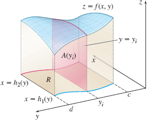
Figure 15 provides justification for Fubini’s Theorem for a \(y\)-simple region \(R\) when \(z=f(x,y)\ge0\) is continuous on \(R\). The volume \(V\) of the solid under \(z=f(x,y) \) from \(y=c\) to \(y=d\) is given by \[ V=\int_{c}^{d}A(y)\,{\it dy} \]
Since this volume \(V\) is also given by \(V=\iint\limits_{\kern-3ptR} f(x,y)\,dA,\) we have \begin{equation} V=\displaystyle\iint\limits_{\kern-3ptR} f(x,y)\,dA=\int_{c}^{d}A(y)\,dy\tag {2} \end{equation}
But \(A(y_{i})\) is the area of the plane region under the surface \( z=f(x,y_{i})\) from \(x=h_{1}(y_{i})\) to \(x=h_{2}(y_{i})\). That is, \begin{equation*} A(y)=\int_{h_{1}(y)}^{h_{2}(y)}f(x,y)\,dx \end{equation*}
where \(y\) is held constant. By substituting \( \int_{h_{1}(y)}^{h_{2}(y)}f(x,y)\,{\it dx}\) for \(A(y)\) in the volume formula (2), we find \[ V=\displaystyle\iint\limits_{\kern-3ptR} f(x,y)\,dA=\int_{c}^{d}\underset{\color {#0066A7}{\hbox{\(A(y)\)}}}{ \underbrace{\left[ \int_{h_{1}(y)}^{h_{2}(y)}f(x,y)\,dx\right] }}dy \]
2 Use Fubini’s Theorem for an \(y\)-Simple RegionPrinted Page 916
916
EXAMPLE 2Use Fubini’s Theorem for an \(y\)-Simple Region
Find \(\iint\limits_{\kern-3ptR}3x^{2}y\,dA\) if \(R\) is the region bounded by the smooth curves \(x=\sqrt{y}\) and \(x=-y\), and the line \(y=1\).
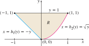
Solution We begin by graphing the region \(R\). See Figure 16. Observe that \(R\) is a closed, bounded region that is \(y\)-simple, where \( h_{1}(y)=-y\) and \(h_{2}(y)=\sqrt{y}\), \(0\leq y\leq 1\). Using Fubini’s Theorem for a \(y\)-simple region, we have \begin{eqnarray*} \displaystyle\iint\limits_{\kern-3ptR}3x^{2}y\,dA &=&\int_{0}^{1}\left[ \int_{-y}^{\sqrt{y}}3x^{2}y\,dx\right] \! dy=\int_{0}^{1}\big[ y\,x^{3}\big] _{-y}^{\sqrt{y}}\,dy\\[4pt] &=&\int_{0}^{1}y(y^{3/2}+y^{3})\,dy=\int_{0}^{1}(y^{5/2}+y^{4})\,dy \\[4pt] &=&\left[ \dfrac{y^{7/2}}{7/2}+\dfrac{y^{5}}{5}\right] _{0}^{1}=\dfrac{2}{7}+\dfrac{1}{5}=\dfrac{17}{35} \end{eqnarray*}
NOW WORK
When the region \(R\) is both \(x\)-simple and \(y\)-simple, we can choose the order of integration. In some cases, integration in one order uses simpler techniques than the techniques needed to integrate in the opposite order.
EXAMPLE 3Finding a Double Integral over a Region That Is \(x \)-Simple and \(y\)-Simple
Find \(\iint\limits_{\kern-3ptR} e^{y^{2}}\,dA\), where \(R\) is the region shown in Figure 17.
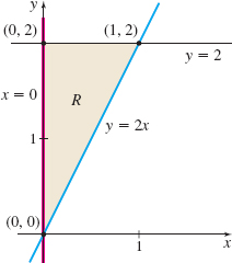
Solution The region \(R\) is both \(x\)-simple and \(y\)-simple.
If we treat \(R\) as \(x\)-simple, then the bottom boundary of \(R\) is \(y=2x\) and the top boundary is \(y=2,\) \(0\leq x\leq 1.\) Then by Fubini’s Theorem, \[ \displaystyle\iint\limits_{\kern-3ptR} e^{y^{2}} dA=\int_{0}^{1}\left[ \int_{2x}^{2}e^{y^{2}} dy \right] dx \]
We cannot find \(\int_{2x}^{2}e^{y^{2}} dy\) using the Fundamental Theorem of Calculus since this integral is not expressible in terms of elementary functions.
So, we consider the region \(R\) as \(y\)-simple. Then the left boundary of \(R\) is \(x=0\) and the right boundary is \(x=\dfrac{y}{2},\) where \(0\leq y\leq 2.\) Then by Fubini’s Theorem, \begin{eqnarray*} \displaystyle\iint\limits_{\kern-3ptR} e^{y^{2}}dA &=&\int_{0}^{2}\left[ \int_{0}^{y/2}e^{y^{2}} dx\right] \! dy=\int_{0}^{2} e^{y^{2}} \big[x\big] _{0}^{y/2}\,dy=\int_{0}^{2}\dfrac{y}{2}e^{y^{2}} dy \notag \\[5pt] &=&\dfrac{1}{2}\int_{0}^{2}ye^{y^{2}} dy=\dfrac{1}{2}\left[ \dfrac{e^{y^{2}} }{2}\right] _{0}^{2}=\dfrac{1}{4}(e^{4}-1) \end{eqnarray*}
NOW WORK
3 Work with Properties of Double IntegralsPrinted Page 917
917
Double integrals have properties very similar to properties of single integrals.
NEED TO REVIEW?
Properties of single integrals are discussed in Section 5.4, pp. 369-374.
THEOREM Properties of Double Integrals
Suppose \(f\) and \(g\) are functions of two variables that are continuous on a closed, bounded region \(R\). Then both \(\displaystyle\iint\limits_{\kern-3ptR} f (x,y) \, dA\) and \(\displaystyle\iint\limits_{\kern-3ptR} g(x,y) \, dA\) exist.
- \(\displaystyle\iint\limits_{\kern-3ptR} [f(x,y)\pm g(x,y)]\,dA=\displaystyle\iint\limits_{\kern-3ptR} f(x,y)\,dA\pm \displaystyle\iint \limits_{\kern-3ptR} g(x,y)\,dA\).
- \(\displaystyle\iint\limits_{\kern-3ptR} cf(x,y)\,dA=c\displaystyle\iint\limits_{\kern-3ptR} f(x,y)\,dA,\) where \(c\) is a constant.
- If \(R\) consists of two subregions, \(R_{1}\) and \(R_{2}\), that have no points in common except for points lying on portions of their common boundary, then \[ \displaystyle\iint\limits_{\kern-3ptR} f(x,y)\,dA=\displaystyle\iint\limits_{\kern-3ptR_{1}} f(x,y)\,dA+\displaystyle\iint \limits_{\kern-3ptR_{2}} f(x,y)\,dA \]
EXAMPLE 4Using Properties of Double Integrals
If \(R\) is a closed, bounded region, then
- (a) \(\displaystyle\iint\limits_{\kern-3ptR} ( x^{2}y+\sin x\cos y) \,dA=\displaystyle\iint\limits_{\kern-3ptR} x^{2}y\,dA+\displaystyle\iint\limits_{\kern-3ptR}\sin x\cos y\,dA\)
- (b) \(\displaystyle\iint\limits_{\kern-3ptR} 8( x^{2}+y^{2})\, dA=8\displaystyle\iint\limits_{\kern-3ptR} ( x^{2}+y^{2})\, dA\)
NOW WORK
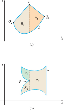
The third property of double integrals is useful when the closed, bounded region \(R\) is neither \(x\)-simple nor \(y\)-simple. In such cases, it may be possible to partition \(R\) into subregions, each of which is \(x\)-simple or \(y\) -simple. Figure 18 illustrates how this can be done.
In Figure 18(a), \(R\) is neither \(x\)-simple nor \(y\)-simple. It is not \(x\) -simple because of the corner at the point \(P.\) It is not \(y\)-simple because of the corners at \(Q_1\) and \(Q_2\). However, if we draw a vertical line through \(P,\) we partition \(R\) into two nonoverlapping subregions \(R_{1}\) and \(R_{2}\), each of which is \(x\)-simple.
In Figure 18(b), the region \(R\) is neither \(x\)-simple nor \(y\)-simple. However, if we draw a vertical line that passes through the corner \(P\) of the left boundary, we partition \(R\) into three nonoverlapping subregions \( R_{1}, \) \(R_{2},\) and \(R_{3,}\) each of which is \(x\)-simple.
EXAMPLE 5Using Properties of Double Integrals
Find \(\displaystyle\iint\limits_{\kern-3ptR} x^{2}y\,dA,\) where \(R\) is the region enclosed by the lines \(y=x,\) \(y=x+2\), \(y=-x+2,\) and \(y=-x+4.\)
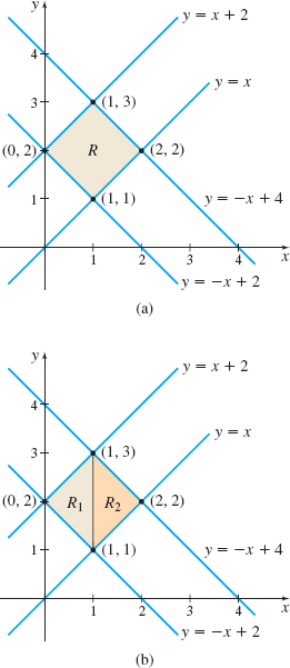
Solution We begin by graphing the region \(R\) as shown in Figure 19(a). We observe that \(R\) is a closed, bounded region, but it is neither \(x\) -simple nor \(y\)-simple. It is not \(x\)-simple due to the corners at \(( 1,3) \) and \((1,1) .\) It is not \(y\)-simple due to the corners at \(( 0,2) \) and \((2,2) .\) But we can partition \(R\) into subregions \(R_{1}\) and \(R_{2}\), both of which are \(x\)-simple, by drawing a vertical line from \(( 1,3) \) to \(( 1,1) \). See Figure 19(b). The subregion \(R_{1}\) is \(x\)-simple with \( g_{1}(x) =-x+2\); \(g_{2}(x)=x+2\), \(0\leq x\leq 1.\) The subregion \(R_{2}\) is \(x\)-simple with \(h_{1}(x) =x\); \( h_{2}(x)=-x+4\), \(1\leq x\leq 2.\) Then \begin{eqnarray*} \displaystyle\iint\limits_{\kern-3ptR}x^{2}y\,{\it dA} &=&\displaystyle\iint\limits_{\kern-3ptR_{1}}x^{2}y\,{\it dA}+\displaystyle\iint\limits_{\kern-3ptR_{2}}x^{2}y\,{\it dA}\\[4pt] &=&\int_{0}^{1} \left[ \int_{-x+2}^{x+2}x^{2}y\,{\it dy}\right] \! {\it dx}+\int_{1}^{2} \left[ \int_{x}^{-x+4}x^{2}y\,{\it dy}\right] \! {\it dx} \notag \\[4pt] &=&\int_{0}^{1} x^{2}\left[\dfrac{y^{2}}{2}\right] _{-x+2}^{x+2}\,{\it dx}+ \int_{1}^{2} x^{2}\left[\dfrac{y^{2}}{2}\right] _{x}^{-x+4}\,{\it dx} \notag \\[4pt] &=&\dfrac{1}{2}\int_{0}^{1}x^{2}\left[ (x+2) ^{2}-\left( -x+2\right) ^{2}\right] \! {\it dx}+\dfrac{1}{2}\int_{1}^{2}x^{2}\left[ \left( -x+4\right) ^{2}-x^{2}\right] \! {\it dx} \notag \\[4pt] &=&\dfrac{1}{2}\int_{0}^{1}8x^{3}\,{\it dx}+\dfrac{1}{2}\int_{1}^{2}(-8x^{3}+16x^{2}) \,{\it dx} \notag \\[4pt] &=&4\left[\dfrac{x^4}{4}\right]^1_0 - 4\left[\dfrac{x^4}{4}\right]^2_1 + 8 \left[\dfrac{x^3}{3}\right]^2_1 = 1-15+\dfrac{56}{3}=\dfrac{14}{3} \end{eqnarray*}
918
In Example 5, we could have also partitioned \(R\) into two subregions, both of which are \(y\)-simple.
NOW WORK
Example 5 using \(y\)-simple subregions.
4 Use Double Integrals to Find Area and VolumePrinted Page 918
Double integrals can be used to find the area of a closed, bounded region \(R\). To find area using a double integral, let \(f(x,y)=1\) and use the theorem for finding the volume under a surface. The volume under the surface \(f(x,y)=1\) and over the region \(R\) is numerically equal to the area of the region \(R\). That is, \[\bbox[5px, border:1px solid black, #F9F7ED]{\bbox{ \hbox{Area of the region } R=\displaystyle\iint\limits_{\kern-3ptR}\,{\it dA} }} \]
EXAMPLE 6Using a Double Integral to Find the Area of a Region
Use a double integral to find the area \(A\) of the region \(R\) in the first quadrant enclosed by the parabola \(y=6x-x^{2}\) and the line \(y=4x-8\).
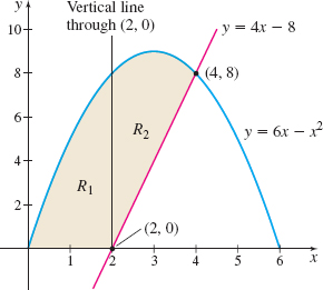
Solution The graph of the region \(R\) is shown in Figure 20. Notice that \(R\) is neither \(x\)-simple nor \(y\)-simple. It is not \(x\)-simple because of the corner at \((2,0)\); it is not \(y\)-simple because of the corner at \((4,8)\). If we partition \(R\) by drawing a vertical line through the point \((2,0)\), we obtain two \(x\)-simple subregions \(R_{1}\) and \(R_{2}\). Then the area \(A\) of the region \(R\) is \begin{eqnarray*} A&=&\displaystyle\iint\limits_{\kern-3ptR}\,{\it dA}=\displaystyle\iint\limits_{\kern-3ptR_{1}}\,{\it dA}+\displaystyle\iint\limits_{\kern-3ptR_{2}}\,{\it dA}= \int_{0}^{2}\left[ \int_{0}^{6x-x^{2}} {\it dy} \right]\! {\it dx}+\int_{2}^{4}\left[ \int_{4x-8}^{6x-x^{2}} {\it dy}\right]\! {\it dx} \notag \\[4pt] & =&\int_{0}^{2}(6x-x^{2})\,{\it dx}+\int_{2}^{4}(-x^{2}+2x+8)\,{\it dx} \notag \\[4pt] & =&\left[ 3x^{2}-\dfrac{x^{3}}{3}\right] _{0}^{2}+\left[ -\dfrac{x^{3}}{3} +x^{2}+8x\right] _{2}^{4}= \dfrac{56}{3}\hbox{ square units} \end{eqnarray*}
NOW WORK
919
EXAMPLE 7Using a Double Integral to Find the Volume of a Solid
Find the volume \(V\) of the solid in the first octant enclosed by the plane \(x+y+z=1\).
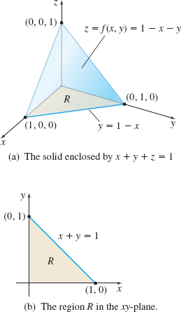
Solution Figure 21(a) shows the solid in the first octant enclosed by the plane \(x+y+z=1\). The volume \(V\) of the solid lies under the plane \(z=f(x,y) =1-x-y\) and above the region \(R\) in the \(xy\)-plane bounded by the lines \(x=0,\) \(y=0,\) and \(x+y=1.\) See Figure 21(b). The region \(R\) is \(x\)-simple and \(y\)-simple. If we treat \(R\) as \(x\)-simple, then \(y\) varies from \(y=0\) to \(y=1-x\), \(0\leq x \leq 1\). The volume \(V\) of the solid is \begin{eqnarray*} V=\displaystyle\iint\limits_{\kern-3ptR}f(x,y) \,{\it dA}& =&\int_{0}^{1}\left[ \int_{0}^{1-x}(1-x-y)\,{\it dy}\right]\! {\it dx}=\int_{0}^{1}\left[ ( 1-x) y- \dfrac{y^{2}}{2}\right] _{0}^{1-x} {\it dx}\\[5pt] &=&\int_{0}^{1}\left[ (1-x)^{2}-\dfrac{(1-x)^{2}}{2}\right] \! {\it dx} \\[5pt] & =&\dfrac{1}{2}\int_{0}^{1}(1-x)^{2}\,{\it dx}=\dfrac{1}{2}\left[ x-x^{2}+\dfrac{x^{3} }{3}\right] _{0}^{1}=\dfrac{1}{6}\hbox{ cubic unit} \end{eqnarray*}
NOW WORK
EXAMPLE 8Using a Double Integral to Find the Volume of a Solid
Find the volume \(V\) common to the two cylinders \(x^{2}+y^{2}=1\) and \( x^{2}+z^{2}=1\).
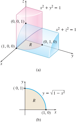
Solution Each cylinder has radius \(1\); their axes are perpendicular to each other and lie on the \(z\)-axis and \(y\)-axis, respectively. Figure 22(a) shows the portion of the solid lying in the first octant. If we find the volume of this portion of the solid, then since the volume in each octant is the same, the volume \(V\) is eight times the volume in the first octant. That is, if \(z=f(x,y) =\sqrt{1-x^{2}},\) then \[ V=8\displaystyle\iint\limits_{\kern-3ptR}f(x,y) \,{\it dA}=8\displaystyle\iint\limits_{\kern-3ptR}(1-x^{2})^{1/2}\, {\it dA} \]
where \(R\) is the region in the first quadrant inside the circle \(x^{2}+y^{2}=1.\) See Figure 22(b).
Consider the integrand. It is simpler to integrate with respect to \(y\) first. (Do you see why?) So, we treat \(R\) as an \(x\)-simple region. (If this approach fails, we would try treating \(R\) as a \(y\)-simple region.) If \(R\) is \(x\)-simple, then \(y\) varies from \(0\) to \((1-x^{2})^{1/2}\), \(0\leq x\leq 1\). The volume \(V\) is \begin{eqnarray*} V &=&8\displaystyle\iint\limits_{\kern-3ptR}(1-x^{2})^{1/2}\, {\it dy}\,{\it dx}=8\int_{0}^{1}\left[ \int_{0}^{ \sqrt{1-x^{2}}}(1-x^{2})^{1/2}\,{\it dy}\right] \! {\it dx}\\[5pt] &=&8\int_{0}^{1}\Big[ (1-x^{2})^{1/2}y\Big] _{0}^{\sqrt{1-x^{2}}}\,{\it dx} \notag \\[5pt] &=&8\int_{0}^{1}(1-x^{2})\,{\it dx}=8\left[ x-\dfrac{x^{3}}{3}\right] _{0}^{1}= \dfrac{16}{3}\hbox{ cubic units} \end{eqnarray*}