1.3 ContinuityPrinted Page 93
93
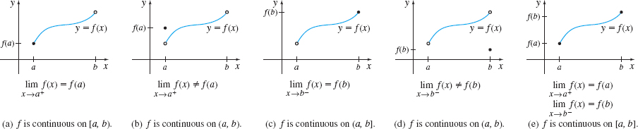
Sometimes \(\lim\limits_{x\rightarrow c}f(x)\) equals \(f(c)\) and sometimes it does not. In fact, \(f(c)\) may not even be defined and yet \(\lim\limits_{x\rightarrow c}f(x)\) may exist. In this section, we investigate the relationship between \(\lim\limits_{x\rightarrow c}f(x)\) and \(f(c)\). Figure 21 shows some possibilities.
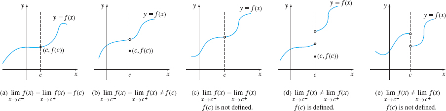
Of these five graphs, the “nicest” one is Figure 21(a). There, \(\lim\limits_{x\rightarrow c}f(x)\) exists and is equal to \(f(c)\). Functions that have this property are said to be continuous at the number \(c\). This agrees with the intuitive notion that a function is continuous if its graph can be drawn without lifting the pencil. The functions in Figures 21(b)-(e) are not continuous at \(c\), since each has a break in the graph at \(c\). This leads to the definition of continuity at a number.
DEFINITION Continuity at a Number
A function \(f\) is continuous at a number \(c\) if the following three conditions are met:
- \(f(c)\) is defined (that is, \(c\) is in the domain of \(f\))
- \(\lim\limits_{x\rightarrow c}f(x)\) exists
- \(\lim\limits_{x\rightarrow c}f(x)=f(c)\)
If any one of these three conditions is not satisfied, then the function is discontinuous at \(c\).
1 Determine Whether a Function Is Continuous at a NumberPrinted Page 93
EXAMPLE 1Determining Whether a Function Is Continuous at a Number
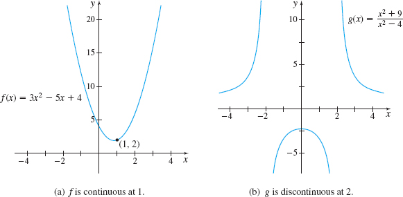
- (a) Determine whether \(f(x)=3x^{2}-5x+4\) is continuous at \(1\).
- (b) Determine whether \(g(x)=\dfrac{x^{2}+9}{x^{2}-4}\) is continuous at \(2\).
Solution (a) We begin by checking the conditions for continuity. First, \(1\) is in the domain of \(f\) and \(f( 1) =2.\) Second, \(\lim\limits_{x\rightarrow 1}f(x)=\lim\limits_{x\rightarrow 1}(3x^{2}-5x+4)=2,\) so \(\lim\limits_{x\rightarrow 1}f( x) \) exists. Third, \(\lim\limits_{x\rightarrow 1}f( x) =f( 1)\). Since the three conditions are met, \(f\) is continuous at \(1\).
(b) Since \(2\) is not in the domain of \(g\), the function \(g\) is discontinuous at \(2\).
94
Figure 22 shows the graphs of \(f\) and \(g\) from Example 1. Notice that \(f\) is continuous at \(1\), and its graph is drawn without lifting the pencil. But the function \(g\) is discontinuous at \(2\), and to draw its graph, you must lift your pencil at \(x=2\).
NOW WORK
EXAMPLE 2Determining Whether a Function Is Continuous at a Number
Determine if \(f(x)=\dfrac{\sqrt{x^{2}+2}}{x^{2}-4}\) is continuous at the numbers \(-2\), \(0\), and \(2\).
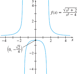
Solution The domain of \(f\) is \(\{x|x\neq -2\), \(x\neq 2\}\). Since \(f\) is not defined at \(-2\) and \(2\), the function \(f\) is not continuous at \(-2\) and at \(2\). The number \(0\) is in the domain of \(f\). That is, \(f\) is defined at \(0\), and \( f(0)=-\dfrac{\sqrt{2}}{4}\). Also, \begin{eqnarray*} \lim_{x\rightarrow 0}f(x)&=&\lim_{x\rightarrow 0}\frac{\sqrt{x^{2}+2}}{ x^{2}-4}=\frac{\lim\limits_{x\rightarrow 0}\sqrt{x^{2}+2}}{ \lim\limits_{x\rightarrow 0}(x^{2}-4)}=\frac{\sqrt{\lim\limits_{x\rightarrow 0}(x^{2}+2)}}{\lim\limits_{x\rightarrow 0}x^{2}-\lim\limits_{x\rightarrow 0}4 }\\[5pt] &=&\frac{\sqrt{0+2}}{0-4}=-\frac{\sqrt{2}}{4}=f(0) \end{eqnarray*}
The three conditions of continuity at a number are met. So, the function \(f\) is continuous at \(0\).
Figure 23 shows the graph of \(f\).
NOW WORK

EXAMPLE 3Determining Whether a Piecewise-Defined Function Is Continuous
Determine if the function \begin{equation*} f(x)=\left\{ \begin{array}{c@{\qquad}l} \dfrac{x^{2}-9}{x-3} & \hbox{if }x\lt 3 \\ 9 & \hbox{if }x=3 \\[5pt] x^{2}-3 & \hbox{if }x>3 \end{array} \right. \end{equation*}
is continuous at \(3\).
95
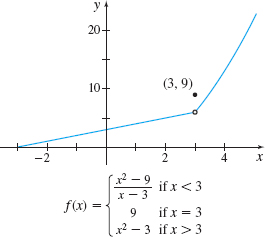
Solution Since \(f(3)=9\), the function \(f\) is defined at \(3\). To check the second condition, we investigate the one-sided limits. \[ \begin{eqnarray*} \lim_{x\rightarrow 3^{-}}f(x) &=&\lim_{x\rightarrow 3^{-}}\frac{x^{2}-9}{x-3 }=\lim_{x\rightarrow 3^{-}}\frac{( x-3) ( x+3) }{x-3} \underset{\underset{\color{#0066A7}{\hbox{Divide out \(x-3\)}}}{\color{#0066A7}{\uparrow}}} {=}\lim_{x\rightarrow 3^{-}}(x+3)=6 \\ \lim_{x\rightarrow 3^{+}}f(x) &=&\lim_{x\rightarrow 3^{+}} (x^{2}-3) =9-3=6 \end{eqnarray*} \]
Since \(\lim\limits_{x\rightarrow 3^{-}}f(x)=\lim\limits_{x\rightarrow 3^{+}}f(x)\), then \(\lim\limits_{x\rightarrow 3}f(x)\) exists. But, \(\lim\limits_{x\rightarrow 3}f(x)=6\) and \(f(3)=9\), so the third condition of continuity is not satisfied. The function \(f\) is discontinuous at \(3\).
Figure 24 shows the graph of \(f\).
NOW WORK
The discontinuity at \(c=3\) in Example 3 is called a removable discontinuity because we can redefine \(f\) at the number \(c\) to equal \(\lim\limits_{x\rightarrow c}f(x)\) and make \(f\) continuous at \(c\). So, in Example 3, if \(f(3)\) is redefined to be \(6\), then \(f\) would be continuous at \(3\).
DEFINITION Removable Discontinuity
Let \(f\) be a function that is defined everywhere in an open interval containing \(c\), except possibly at \(c\). The number \(c\) is called a removable discontinuity of \(f\) if the function is discontinuous at \(c\) but \(\lim\limits_{x\rightarrow c}f( x) \) exists. The discontinuity is removed by defining (or redefining) the value of \(f\) at \(c\) to be \(\lim\limits_{x\rightarrow c}f( x)\).
NOW WORK
NEED TO REVIEW?
The floor function is discussed in Section P.2, p. 17.
EXAMPLE 4Determining Whether a Function Is Continuous at a Number
Determine if the floor function \(f(x)=\lfloor x\rfloor\) is continuous at \(1\).
Solution The floor function \(f( x) =\lfloor x\rfloor =\) the greatest integer \(\leq x\). The floor function \(f\) is defined at \(1\) and \(f(1)=1\). But \begin{equation*} \lim_{x\rightarrow 1^{-}}f(x)=\lim_{x\rightarrow 1^{-}}\lfloor x\rfloor =0\hbox{ and }\lim_{x\rightarrow 1^{+}}f(x)=\lim_{x\rightarrow 1^{+}}\lfloor x\rfloor =1 \end{equation*}
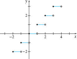
So, \(\lim\limits_{x\rightarrow 1}\lfloor x\rfloor\) does not exist. Since \(\lim\limits_{x\rightarrow 1}\lfloor x\rfloor\) does not exist, \(f\) is discontinuous at \(1\).
See Figure 25 for the graph of the floor function.
As Figure 25 illustrates, the floor function is discontinuous at each integer. Also, none of the discontinuities of the floor function is removable. Since at each integer the value of the floor function “jumps” to the next integer, without taking on any intermediate values, the discontinuity at integer values is called a jump discontinuity.
NOW WORK
We have defined what it means for a function \(f\) to be continuous at a number. Now we define one-sided continuity at a number.
DEFINITION One-Sided Continuity at a Number
Let \(f\) be a function defined on the interval \((a,c]\). Then \(f\) is continuous from the left at the number \(c\) if \begin{equation*} \lim_{^{{}}x\rightarrow c^{-}}f(x)=f(c) \end{equation*}
Let \(f\) be a function defined on the interval \([c,b)\). Then \(f\) is continuous from the right at the number \(c\) if \begin{equation*} \lim_{^{{}}x\rightarrow c^{+}}f(x)=f(c) \end{equation*}
96
In Example 4, we showed that the floor function \(f( x) = \lfloor x\rfloor \) is discontinuous at \(x=1\). But since \begin{equation*} f(1)=\,\lfloor 1\rfloor =1\hbox{ and }\lim_{x\rightarrow 1^{+}}f(x)=\,\lfloor x\rfloor =1 \end{equation*}
the floor function is continuous from the right at \(1\). In fact, the floor function is discontinuous at each integer \(n\), but it is continuous from the right at every integer \(n\). (Do you see why?)
2 Determine Intervals on Which a Function Is ContinuousPrinted Page 96
So far, we have considered only continuity at a number \(c\). Now, we use one-sided continuity to define continuity on an interval.
DEFINITION Continuity on an Interval
- A function \(f\) is continuous on an open interval \((a,b)\) if \(f\) is continuous at every number in \((a,b)\).
- A function \(f\) is continuous on an interval \([a,b)\) if \(f\) is continuous on the open interval \((a,b)\) and continuous from the right at the number \(a\).
- A function \(f\) is continuous on an interval \(( a,b]\) if \(f\) is continuous on the open interval \((a,b)\) and continuous from the left at the number \(b\).
- A function \(f\) is continuous on a closed interval \([a,b]\) if \(f\) is continuous on the open interval \((a,b)\), continuous from the right at \(a\), and continuous from the left at \(b\).
Figure 26 gives examples of graphs over different types of intervals.
For example, the graph of the floor function \(f(x)= \lfloor x\rfloor\) in Figure 25 illustrates that \(f\) is continuous on every interval \([n,n+1)\), \(n\) an integer. In each interval, \(f\) is continuous from the right at the left endpoint \(n\) and is continuous at every number in the open interval \((n,n+1) \).
EXAMPLE 5Determining Whether a Function Is Continuous on a Closed Interval
Is the function \(f(x)=\sqrt{4-x^{2}}\) continuous on the closed interval \([-2,2]\)?
Solution The domain of \(f\) is \(\{x|-2\leq x\leq 2\}\). So, \(f\) is defined for every number in the closed interval \([-2,2]\).
For any number \(c\) in the open interval \((-2,2)\), \begin{equation*} \lim_{x\rightarrow c}f(x)=\lim_{x\rightarrow c}\sqrt{4-x^{2}}=\sqrt{ \lim\limits_{x\rightarrow c}(4-x^{2})}=\sqrt{4-c^{2}}=f(c) \end{equation*}
So, \(f\) is continuous on the open interval \((-2,2)\).
97
To determine whether \(f\) is continuous on \([-2,2]\), we investigate the limit from the right at \(-2\) and the limit from the left at \(2\). Then, \begin{equation*} \lim_{x\rightarrow -2^{+}}f(x)=\lim_{x\rightarrow -2^{+}}\sqrt{4-x^{2}} =0=f(-2) \end{equation*}
So, \(f\) is continuous from the right at \(-2\). Similarly, \begin{equation*} \lim_{x\rightarrow 2^{-}}f(x)=\lim_{x\rightarrow 2^{-}}\sqrt{4-x^{2}} =0=f(2) \end{equation*}
So, \(f\) is continuous from the left at \(2\). We conclude that \(f\) is continuous on the closed interval \([-2,2]\).
NOW WORK
DEFINITION Continuity on a Domain
A function \(f\) is continuous on its domain if it is continuous at every number \(c\) in its domain.
EXAMPLE 6Determining Whether \({f(x)=\sqrt{x^2(x-1)}}\) Is Continuous on Its Domain
Determine if the function \(f(x)=\sqrt{x^{2}(x-1)}\) is continuous on its domain.
Solution The domain of \(f(x)=\sqrt{x^{2}(x-1)}\) is \(\{x|x=0\}\cup \{ x|x\geq 1\}\). We need to determine whether \(f\) is continuous at the number \(0\) and whether \(f\) is continuous on the interval \([ 1,\infty)\).
At the number \(0\), there is an open interval containing \(0\) that contains no other number in the domain of \(f\). [For example, use the interval \(\left( -\dfrac{1}{2},\dfrac{1}{2}\right)\!.]\) This means \(\lim\limits_{x\rightarrow 0}f(x)\) does not exist. So, \(f\) is discontinuous at \(0\).
For all numbers \(c\) in the open interval \((1,\infty )\) we have \begin{equation*} f(c)=\sqrt{c^{2}(c-1)} \end{equation*}
and \begin{equation*} \lim_{x\rightarrow c}\sqrt{x^{2}(x-1)}=\sqrt{\lim\limits_{x\rightarrow c} [x^{2}(x-1)] }=\sqrt{c^{2}(c-1)}=f(c) \end{equation*}
So, \(f\) is continuous on the open interval \((1,\infty )\).
Now, at the number \(1\), \begin{equation*} f(1)=0\hbox{ and }\lim_{x\rightarrow 1^{+}}\sqrt{x^{2}(x-1)}=0 \end{equation*}
So, \(f\) is continuous from the right at \(1\).
The function \(f(x)=\sqrt{x^{2}(x-1)}\) is continuous on the interval \([1,\infty )\), but it is discontinuous at \(0\). So, \(f\) is not continuous on its domain.
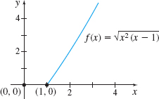
Figure 27 shows the graph of \(f\). The discontinuity at 0 is subtle. It is neither a removable discontinuity nor a jump discontinuity.
When listing the properties of a function in Chapter P, we included the function's domain, its symmetry, and its zeros. Now we add continuity to the list by asking, “Where is the function continuous?” We answer this question here for two important classes of functions: polynomial functions and rational functions.
THEOREM
- A polynomial function is continuous for all real numbers.
- A rational function is continuous on its domain.
98
Proof
If \(P\) is a polynomial function, its domain is the set of real numbers. For a polynomial function, \begin{equation*} \lim_{x\rightarrow c}P(x)=P(c) \end{equation*}
for any number \(c\). That is, a polynomial function is continuous at every real number.
If \(R(x)=\dfrac{p(x)}{q(x)}\) is a rational function, then \(p(x)\) and \(q(x)\) are polynomials and the domain of \(R\) is \(\{x|q(x)\neq 0\}\). The Limit of a Rational Function (p. 87) states that for all \(c\) in the domain of a rational function, \[ \begin{equation*} \lim_{x\rightarrow c}R(x)=R( c) \end{equation*} \]
So a rational function is continuous at every number in its domain.
To summarize:
- If a function is continuous on an interval, its graph has no holes or gaps on that interval.
- If a function is continuous on its domain, it will be continuous at every number in its domain; its graph may have holes or gaps at numbers that are not in the domain.
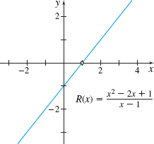
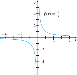
For example, the function \(R( x) =\dfrac{x^{2}-2x+1}{x-1}\) is continuous on its domain \(\{ x|x\neq 1\}\) even though the graph has a hole at \((1,0)\), as shown in Figure 28. The function \(f( x) = \dfrac{1}{x}\) is continuous on its domain \(\{x|x\neq 0\}\), as shown in Figure 29. Notice the behavior of the graph as \(x\) goes from negative numbers to positive numbers.
3 Use Properties of ContinuityPrinted Page 98
So far we have shown that polynomial and rational functions are continuous on their domains. From these functions, we can build other continuous functions.
THEOREM Continuity of a Sum, Difference, Product, and Quotient
If the functions \(f\) and \(g\) are continuous at a number \(c\), and if \(k\) is a real number, then the functions \(f+g,\) \(f-g,\) \(f\cdot g\), and \(kf\) are also continuous at \(c\). If \(g( c) \neq 0,\) the function \(\dfrac{f}{g}\) is continuous at \(c\).
99
The proofs of these properties are based on properties of limits. For example, the proof of the continuity of \(f+g\) is based on the Limit of a Sum property. That is, if \(\lim\limits_{x\rightarrow c}f(x)\) and \(\lim\limits_{x\rightarrow c}g(x)\) exist, then \(\lim\limits_{x\rightarrow c}[ f(x)+g(x)] = \lim\limits_{x\rightarrow c}f(x)+\lim\limits_{x\rightarrow c}g(x)\).
EXAMPLE 7Identifying Where Functions Are Continuous
Determine where each function is continuous:
- (a) \(F(x) = x^{2}+5\) \(-\dfrac{x}{x^{2}+4}\)
- (b) \(G( x) =x^{3}+2x+\dfrac{x^{2}}{x^{2}-1}\)
Solution First we determine the domain of each function.
- (a) \(F\) is the difference of the two functions \(f( x) =x^{2}+5\) and \(g( x) =\dfrac{x}{x^{2}+4}\), each of whose domain is the set of all real numbers. So, the domain of \(F\) is the set of all real numbers. Since \(f\) and \(g\) are continuous on their domains, the difference function \(F\) is continuous on its domain.
- (b) \(G\) is the sum of the two functions \(f( x) =x^{3}+2x\), whose domain is the set of all real numbers, and \(g( x) =\dfrac{x^{2}}{x^{2}-1}\), whose domain is \(\left\{ x|x\neq -1,\hbox{ }x\neq 1\right\}\). Since \(f\) and \(g\) are continuous on their domains, \(G\) is continuous on its domain, \(\left\{ x|x\neq -1,\hbox{ }x\neq 1\right\}\).
NOW WORK
NEED TO REVIEW?
Composite functions are discussed in Section P.3, pp. 25-27.
The continuity of a composite function depends on the continuity of its components.
THEOREM Continuity of a Composite Function
If a function \(g\) is continuous at \(c\) and a function \(f\) is continuous at \(g( c)\), then the composite function \((f\circ g)(x)=f(g(x))\) is continuous at \(c\).
EXAMPLE 8Identifying Where Functions Are Continuous
Determine where each function is continuous:
- (a) \(F(x) =\sqrt{x^{2}+4}\)
- (b) \(G(x) =\sqrt{x^{2}-1}\)
- (c) \(H(x) =\dfrac{x^{2}-1}{x^{2}-4}+\sqrt{x-1}\)
Solution (a) \(F=f\circ g\) is the composite of \(f( x) =\sqrt{x}\) and \(g( x) =x^{2}+4\). \(f\) is continuous for \(x\geq 0\) and \(g\) is continuous for all real numbers. The domain of \(F\) is all real numbers and \(F=( f\circ g) ( x) =\sqrt{x^{2}+4}\) is continuous for all real numbers. That is, \(F\) is continuous on its domain.
(b) \(G\) is the composite of \(f( x) =\sqrt{x}\) and \( g( x) =x^{2}-1\). \(f\) is continuous for \(x\geq 0\) and \(g\) is continuous for all real numbers. The domain of \(G\) is \(\{ x|x\geq 1\} \cup \{ x|x\leq -1\} \) and \(G=( f\circ g) ( x) =\sqrt{x^{2}-1}\) is continuous on its domain.
(c) \(H\) is the sum of \(f( x) =\) \(\dfrac{x^{2}-1}{ x^{2}-4}\) and the function \(g( x) =\sqrt{x-1}\). The domain of \(f\) is \(\{ x|x\neq -2, x\neq 2\} \); \(f\) is continuous on its domain. The domain of \(g\) is \(x\geq 1\). The domain of \(H\) is \(\{ x|1\leq x\lt 2\} \cup \{ x|x>2\}\); \(H\) is continuous on its domain.
NOW WORK
NEED TO REVIEW?
Inverse functions are discussed in Section P.4, pp. 32-37.
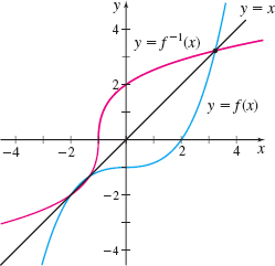
Recall that for any function \(f\) that is one-to-one over its domain, its inverse \(f^{-1}\) is also a function, and the graphs of \(f\) and \(f^{-1}\) are symmetric with respect to the line \(y=x\). It is intuitive that if \(f\) is continuous, then so is \(f^{-1}\). See Figure 30. The following theorem, whose proof is given in Appendix B, confirms this.
100
THEOREM Continuity of an Inverse Function
If \(f\) is a one-to-one function that is continuous on its domain, then its inverse function \(f^{-1}\) is also continuous on its domain.
4 Use the Intermediate Value TheoremPrinted Page 100
Functions that are continuous on a closed interval have many important properties. One of them is stated in the Intermediate Value Theorem. The proof of the Intermediate Value Theorem may be found in most books on advanced calculus.
THEOREM The Intermediate Value Theorem
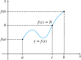
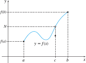
Let \(f\) be a function that is continuous on a closed interval \([a,b]\) and \(f(a)\neq f(b)\). If \(N\) is any number between \(f(a)\) and \(f(b)\), then there is at least one number \(c\) in the open interval \((a,b)\) for which \(f(c)=N\).
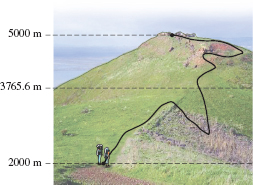
To get a better idea of this result, suppose you climb a mountain, starting at an elevation of \(2000\) meters and ending at an elevation of \(5000\) meters. No matter how many ups and downs you take as you climb, at some time your altitude must be \(3765.6\) meters, or any other number between \( 2000\) and \(5000\).
In other words, a function \(f\) that is continuous on a closed interval \([a,b]\) must take on all values between \(f(a)\) and \(f(b)\). Figure 31 illustrates this and Figure 32 shows why the continuity of the function is crucial.
An immediate application of the Intermediate Value Theorem involves locating the zeros of a function. Suppose a function \(f\) is continuous on the closed interval \([a,b]\) and \(f(a)\) and \(f(b)\) have opposite signs. Then by the Intermediate Value Theorem, there is at least one number \(c\) between \(a\) and \(b\) for which \(f(c)=0\). That is, \(f\) has at least one zero between \(a\) and \(b\).
101
EXAMPLE 9Using the Intermediate Value Theorem
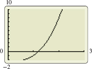
Use the Intermediate Value Theorem to show that \begin{equation*} f(x)=x^{3}+x^{2}-x-2 \end{equation*}
has a zero between \(1\) and \(2\).
Solution Since \(f\) is a polynomial, it is continuous on the closed interval \([1,2]\). Because \(f(1)=-1\) and \(f(2)=8\) have opposite signs, the Intermediate Value Theorem states that \(f(c)=0\) for at least one number \(c\) in the interval \((1,2)\). That is, \(f\) has at least one zero between \(1\) and \(2.\) Figure 33 shows the graph of \(f\) on a graphing utility.
NOW WORK
The Intermediate Value Theorem can be used to approximate a zero by dividing the interval \([a, b]\) into smaller subintervals. There are two popular methods of subdividing the interval \([a, b].\)
The bisection method bisects \([a, b]\), that is, divides \([ a,b]\) into two equal subintervals, and compares the sign of \(f\!\left( \dfrac{b-a}{2}\right)\) to the signs of the previously computed values \(f(a)\) and \(f( b).\) The subinterval whose endpoints have opposite signs is then bisected, and the process is repeated.
The second method divides \([ a,b]\) into \(10\) subintervals of equal length and compares the signs of \(f\) evaluated at each of the eleven endpoints. The subinterval whose endpoints have opposite signs is then divided into \(10\) subintervals of equal length and the process is repeated.
We choose to use the second method because it lends itself well to the table feature of a graphing utility. You are asked to use the bisection method in Problems 103-110.
EXAMPLE 10Using the Intermediate Value Theorem to Approximate a Real Zero of a Function
![]()
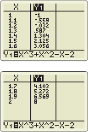
The function \(f(x)=x^{3}+x^{2}-x-2\) has a zero in the interval \((1,2)\). Use the Intermediate Value Theorem to approximate the zero correct to three decimal places.
Solution Using the TABLE feature on a graphing utility, we subdivide the interval \([1,2]\) into \(10\) subintervals, each of length \(0.1\). Then we find the subinterval whose endpoints have opposite signs, or the endpoint whose value equals \(0\) (in which case, the exact zero is found). From Figure 34, since \(f ( 1.2) =-0.032\) and \(f (1.3) =0.587\), by the Intermediate Value Theorem, a zero lies in the interval \(( 1.2,1.3)\). Correct to one decimal place, the zero is \(1.2\).
Repeat the process by subdividing the interval \([ 1.2,1.3]\) into \(10\) subintervals, each of length \(0.01.\) See Figure 35. We conclude that the zero is in the interval \((1.20, 1.21)\), so correct to two decimal places, the zero is \(1.20\).
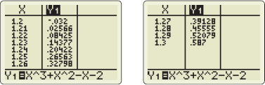
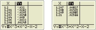
Now subdivide the interval \(\left[ 1.20,1.21\right]\) into \(10\) subintervals, each of length \(0.001.\) See Figure 36.
We conclude that the zero of the function \(f\) is \(1.205,\) correct to three decimal places.
102
Notice that a benefit of the method used in Example 10 is that each additional iteration results in one additional decimal place of accuracy for the approximation.