13.1 Inference About the Slope of the Regression Line
 This page includes Video Technology Manuals
 This page includes Statistical Videos
OBJECTIVES By the end of this section, I will be able to …
- Explain the regression model and the regression model assumptions.
- Perform the hypothesis test for the slope β1 of the population regression equation.
- Construct confidence intervals for the slope β1.
- Use confidence intervals to perform the hypothesis test for the slope β1.
1 The Regression Model and the Regression Assumptions
Before we learn about the regression model and assumptions, let us review the correlation and regression topics that we learned in Chapter 4. Recall that the regression line approximates the linear relationship between two continuous variables and is described by the regression equation ˆy=b1x+b0, where b1 is the slope of the regression line, b0 is the y intercept, x represents the predictor variable, y represents the response variable, and ˆy represents the estimated or predicted y-value.
EXAMPLE 1 Review of regression topics
textms
The Nielsen company has reported that the number of text messages that a person sends tends to decrease with age. Table 1 contains a random sample of 10 people, along with their age and the number of text messages they sent on the previous day.
- Construct and interpret a scatterplot of the response variable y versus the predictor variable x.
- Calculate and interpret the correlation coefficient r.
- Compute the regression equation ˆy=b1x+b0. Interpret the meaning of the y intercept b0 and the slope b1 of the regression equation.
- Predict the number of text messages sent by a 20-year-old person, and calculate the prediction error (residual).
| x=Age | y=Text messages | x=Age | y=Text messages |
|---|---|---|---|
| 18 | 35 | 28 | 16 |
| 20 | 29 | 30 | 19 |
| 22 | 27 | 32 | 12 |
| 24 | 28 | 34 | 8 |
| 26 | 19 | 36 | 8 |
You may want to refer to Section 4.1 for (a) and (b), and Section 4.2 for (c) and (d).
Solution
- The number of messages depends on age, and not vice versa, so the predictor variable x is age and the response variable y is messages. Also, note that in (d) we are trying to predict the number of text messages, which tells us that messages is the response variable y because we never try to predict the known value of x. The TI-83/84 scatterplot is shown in Figure 1. As age increases, the number of messages tends to decrease.Page 717
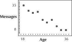 FIGURE 1 TI-83/84 scatterplot of messages versus age.
 - Figure 2 shows the correlation coefficient r≈−0.9701, calculated by the TI-83/84. Age and messages are negatively correlated. An increase in age is associated with a decrease in the number of messages.
Figure 2 shows that a=b1=−1.5 and b=b0=60.6, and thus the regression equation is
ˆy=b1x+b0=(−1.5)(age)+60.6
We can interpret b0 and b1 as follows:
- The y intercept b0=60.6 is the estimated number of text messages sent by someone aged x=0, which does not make sense because this value x=0 lies far below the minimum value of x and therefore represents extreme extrapolation.
- The slope b1=−1.5 means there is an estimated decrease of 1.5 in the number of text messages for each additional year of age.
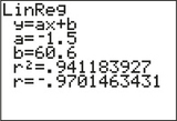 FIGURE 2 TI-83/84 correlation and regression results.
For a 20-year-old person, the estimated number of daily text messages is
ˆy=b1x+b0=(−1.5)(20)+60.6=30.6
The actual number of text messages sent by our 20-year-old in Table 1 is y=29. Our prediction from (c) is ˆy=30.6. Thus, our prediction error (or residual) is: (y−ˆy)=(29−30.6)=−1.6. Our 20-year-old sent slightly fewer text messages than expected.
YOUR TURN#1
The table contains the age (x) and score in a video game (y) for a random sample of five young people.
- Construct and interpret a scatterplot of the response variable y versus the predictor variable x.
- Calculate and interpret the correlation coefficient r.
- Compute the regression equation ˆy=b1x+b0. Interpret the meaning of the y intercept b0 and the slope b1 of the regression equation.
- Predict the score for a 22-year old person, and calculate the prediction error (residual).
(The solutions are shown in Appendix A.)
| Age (x) | Score (y) |
|---|---|
| 14 | 80 |
| 16 | 90 |
| 18 | 90 |
| 20 | 90 |
| 22 | 100 |
Example 1 and our work in Chapter 4 on regression represented descriptive statistics. Next, we turn to learning about inference in regression.
Note that the regression equation ˆy=b1x+b0=(−1.5)(age)+60.6 depends on the sample. It is likely that a second sample will differ from the first, giving us a different regression line and different values for b0 and b1. In fact, for every different sample, b0 and b1 take different values because b0 and b1 are sample statistics. However, every sample comes from a population. We do not have data on the entire population, so we are not able to calculate the population regression equation. The y intercept β0 and slope β1 of the population regression equation are unknown population parameters, just as μ and p are parameters in other contexts. The values of β0 and β1 are unknown, so we need to perform inference to learn about them.
The regression model may be used to approximate the relationship between the predictor variable x and the response variable y for the entire population of (x,y) pairs.
Note that there is no “hat” on the y in the population regression equation because the equation represents a model of the relationship between the actual values of x and y, not an estimate of y.
Regression Model
The population regression equation is defined as
y=β1x+β0+ε
where β0 is the y intercept of the population regression line, β1 is the slope of the population regression line, and ε is the error term.
The 20-year-old in Table 1 sent 29 text messages. Suppose another 20-year-old sent 30 messages, so that both texters had age x=20, but different values of y:y=29 and y=30. Then it would be impossible to draw a single regression line to pass through both (x=20,y=29) and (x=20,y=30). Thus, any linear approximation of the true relationship between x and y will introduce a certain amount of error. This is why the error term ε is needed.
Regression Model Assumptions
The regression model operates under a set of four assumptions that must be valid in order to perform the inference in this section.
Regression Model Assumptions
- Zero-mean assumption. The error term ε is a random variable, with a mean of 0. That is, the expected value of the random variable ε is 0:E(ε)=0.
- Constant variance assumption. The variance of ε, which is denoted as σ2, is the same regardless of the value of x.
- Independence assumption. The values of ε are independent of each other.
- Normality assumption. The error term ε is a normal random variable.
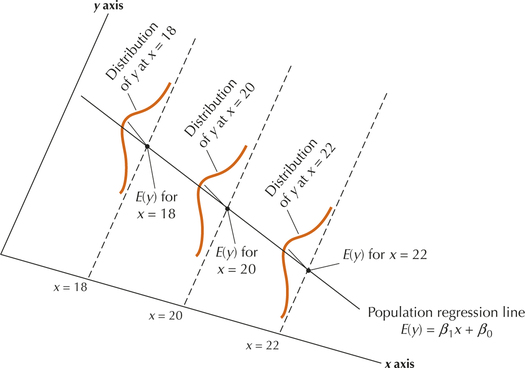
To summarize, for each value of x, the values of y come from a normally distributed population with a mean on the population regression line E(y)=β1x+β0 and constant standard deviation σ2. Figure 3 illustrates how y is distributed for each value of x. Note that each normal curve has the same shape, indicating constant variance for each x.
Verifying the Regression Assumptions
To check the regression model assumptions, we construct two graphs:
- Scatterplot of the residuals (prediction errors, y−ˆy) against the fitted values (fitted values refers to the predicted values, ˆy)
- Normal probability plot of the residuals
Figure 4 shows four types of patterns that might be observed in the residuals versus fitted values plots.
- Plot (a) is a “healthy” plot, displaying no noticeable patterns.
- Plot (b) is a curve, which indicates a violation of the independence assumption. Independence implies that knowing the value of a particular y does not help to predict the value of a different y. However, a curve suggests that knowing the value of a previous y helps in knowing the value of the next y.
- Plot (c) shows a “funnel” pattern, which contradicts the constant variance assumption. The residuals on the left are close together vertically (small variability), whereas the residuals on the right are far apart vertically (large variability).
- Plot (d) shows an increasing pattern that violates the zero-mean assumption. The residuals on the left are all below the midline, so E(y)<β1x+β0, whereas the residuals on the right are all above the midline, so E(y)>β1x+β0.
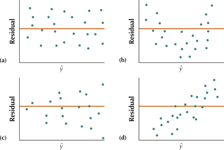 FIGURE 4 Patterns in the residuals versus predicted plots.
Developing Your Statistical Sense
Verifying the Regression Assumptions
With small data sets, it is difficult to ascertain whether or not patterns really exist. Be wary of seeing patterns where none exist. If one or more regression assumptions are violated, we should not proceed with inferential methods such as hypothesis tests or confidence intervals. However, even if one or more regression assumptions are violated, we can still report and interpret the descriptive regression statistics that we learned in Sections 4.2 and 4.3.
EXAMPLE 2 Calculating the residuals and verifying the regression assumptions
For the data in Example 1, do the following:
- Calculate the residuals y−ˆy.
- Verify the regression assumptions.
Solution
- Table 2 contains the x and y data from Table 1, the fitted (predicted) values ˆy, and the residuals y−ˆy.Table 13.3: Table 2 Calculating the residuals
x=Age y=Text messages Fitted (predicted) values ˆy=(−1.5)(age)+60.6
Residuals y−ˆy 18 35 33.6 1.4 20 29 30.6 −1.6 22 27 27.6 −0.6 24 28 24.6 3.4 26 19 21.6 −2.6 28 16 18.6 −2.6 30 19 15.6 3.4 32 12 12.6 −0.6 34 8 9.6 −1.6 36 8 6.6 1.4 - The scatterplot in Figure 5 of the residuals versus fitted values shows no strong evidence of the unhealthy patterns shown in Figure 4. Thus, the independence assumption, the constant variance assumption, and the zero-mean assumption are verified. Also, the normal probability plot of the residuals in Figure 6 indicates no evidence of departures from normality in the residuals. Therefore, we conclude that the regression assumptions are verified.
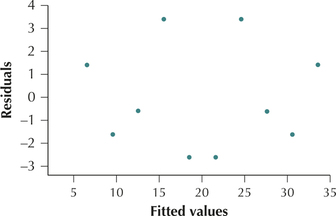 FIGURE 5 Scatterplot of residuals versus fitted values.
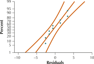 FIGURE 6 Normal probability plot of the residuals.
NOW YOU CAN DO
Exercises 7–14.
YOUR TURN#2
For the data in the Your Turn #1 on page 717, do the following:
- Calculate the residuals y−ˆy. for the regression of score on age.
- Verify the regression assumptions.
(The solutions are shown in Appendix A.)
Once the regression assumptions have been verified, we may (a) perform hypothesis tests, and (b) construct confidence intervals for the population slope β1.
2 Hypothesis Tests for Slope β1
Suppose for a moment that, for the population regression equation y=β1x+β0+ε, the slope β1 equals zero. Then the population regression equation would be
y=(0)x+β0+ε=β0+ε
That is,
- If β1 equals zero, then no relationship exists between x and y, because changing x in the equation y=β0+ε does not affect y.
- If β1 equals any other value, then a linear relationship does exist between x and y.
This idea forms the basis for our inference in this section. To test whether a relationship exists between x and y, we begin with the hypothesis test to determine whether or not β1 equals 0. The hypotheses are
- H0:β1=0 No linear relationship exists between x and y.
- Ha:β1≠0 A linear relationship exists between x and y.
Assuming H0:β1=0 is true, the test statistic tdata for this hypothesis test takes the following form.
Test Statistic tdata
tdata=b1−β1s/√∑(x−ˉx)2=b1−0s/√∑(x−ˉx)2=b1s/√∑(x−ˉx)2
where b1 represents the slope of the regression line, s=√SSEn−2 represents the standard error of the estimate (from Section 4.3), and √∑(x−ˉx)2 is related to the sample variance of the x data (see page 229 in Section 4.3).
 Here, s refers to the standard error of the estimate, not the sample standard deviation.
tdata consists of three quantities: b1, s, and √∑(x−ˉx)2. The next example shows how to calculate tdata by finding these three quantities.
EXAMPLE 3 Calculating tdata
Use the following steps to calculate the test statistic tdata=b1s/√∑(x−ˉx)2 for the data in Table 2:
- Find b1, the slope of the regression line.
- Calculate s, the standard error of the estimate.
- Compute √∑(x−ˉx)2, the numerator of the sample variance of the x data.
Solution
All calculations up to the final result are expressed to nine decimal places.
- From Example 1, the slope of the regression line is b1=−1.5.
Recall from Section 4.3 (page 228) that
s=√SSEn−2=√∑(y−ˆy)2n−2=√∑(residual)2n−2
is the standard error of the estimate. Squaring each residual from Table 2 gives us the squared residuals in Table 3, and the sum of squared residuals, or sum of squares error, equal to
SSE=∑(y−ˆy)2=46.4
Then the standard error of the estimate is
s=√SSEn−2=√46.48≈2.408318916.
Table 13.4: Table 3 Calculating SSEResiduals y−ˆy Squared residuals (y−ˆy)2 1.4 1.96 −1.6 2.56 −0.6 0.36 3.4 11.56 −2.6 6.76 −2.6 6.76 3.4 11.56 −0.6 0.36 −1.6 2.56 1.4 1.96 Sum=46.4 -
s2x=∑(x−ˉx)2n−1
Multiplying each side of the equation by n−1 , we obtain an equation for the quantity ∑(x−ˉx)2:
∑(x−ˉx)2=(n−1)·s2x
The TI-83/84 output from Figure 7 shows that sx=6.055300708 , and, because n=10,
∑(x−ˉx)2= (n−1)· s2x = (9) (6.055300708)2 = 330
Therefore,
tdata = b1s/√∑(x−ˉx)2 = − 1.52.408318916 /√330 ≈ −11.3
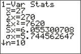 FIGURE 7 Summary statistics for the x (age) data.
Now that we have tdata, we can perform the hypothesis test for the slope β1, as the next example shows using the critical-value method.
EXAMPLE 4 Hypothesis test for slope β1 using the critical-value method
Test whether a linear relationship exists between age and text messages, using the data from Table 1 at level of significance α=0.01.
Solution
The regression assumptions were shown to be valid in Example 2. We may thus proceed with the hypothesis test.
- Step 1 State the hypotheses.
- H0: β1 = 0 No linear relationship exists between age and text messages.
- Ha: β1 ≠ 0 A linear relationship exists between age and text messages.
Step 2 Find the t critical value tcrit and the rejection rule. To find tcrit, use the t distribution table (Table D in the Appendix) for a two-tailed test and degrees of freedom df=n−2. The rejection rule for this two-tailed test is
Reject H0 if tdata ≥ tcrit or tdata ≤ − tcrit
Here, n= 10, so df=8. For level of significance α = 0.01, the t table gives us tcrit = 3.355. We will reject H0 if tdata ≥ 3.335 or tdata ≤ − 3.335.
Step 3 Calculate tdata. From Example 3, we have
tdata = b1s/√∑(x − ˉx)2 ≈ − 11.3
Step 4 State the conclusion and the interpretation. Because tdata ≈ − 11.3 ≤ −3.335, we reject H0. There is evidence, at level of significance α = 0.01, that β1 ≠ 0 and that a linear relationship exists between age and text messages.
NOW YOU CAN DO
Exercises 15–18.
The next example illustrates the steps for performing the hypothesis test for the slope β1 using the p-value method.
EXAMPLE 5 Hypothesis test for the slope β1 using the p-value method and technology
shortmemory
| Time (x) | Score (y) |
|---|---|
| 1 | 9 |
| 1 | 10 |
| 2 | 11 |
| 3 | 12 |
| 3 | 13 |
| 4 | 14 |
| 5 | 19 |
| 6 | 17 |
| 7 | 21 |
| 8 | 24 |
In Section 4.3, we considered a study on short-term memory. Ten subjects were given a set of nonsense words to memorize within a certain amount of time and were later scored on the number of words they could remember. The results are repeated here in Table 4. Use the p-value method and technology to test, using level of significance α = 0.01, whether a linear relationship exists between time and score.
Solution
We begin by verifying the regression assumptions. The scatterplot of the residuals versus the fitted values in Figure 8 shows no strong evidence that the independence assumption, the constant variance assumption, or the zero-mean assumption is violated. Also, the normal probability plot of the residuals in Figure 9 offers evidence of the normality of the results. Therefore, we conclude that the regression assumptions are verified, and proceed with the hypothesis test.
Step 1 State the hypotheses and the rejection rule.
- H0 : β1 = 0 No linear relationship exists between time and score.
- Ha: β1 ≠ 0 A linear relationship exists between time and score.
Page 724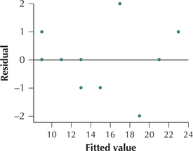 FIGURE 8 Residuals versus fitted values plot.
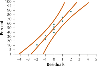 FIGURE 9 Normal probability plot of the residuals.
The rejection rule is: reject H0 if the p-value≤ 0.01.
Step 2 Calculate tdata.
tdata = b1s/√∑(x− ˉx)2
From page 226 in Section 4.3, we have b1= 2. From Example 13 in Chapter 4 on page 228, we have
s= √128 ≈ 1.224744871
From the TI-83/84 summary statistics, we have the standard deviation of the x (time) data to be sx = 2.449489743. Thus, using the relationship we learned in Example 3:
∑(x − ˉx)2= (n − 1) · s2x = (9) 2.4494897432 = 54
Therefore,
tdata = b1s/√∑(x − ˉx)2 ≈ 21.224744871/√54 = 12
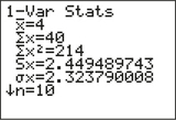 TI-83/84 summary statistics for x (time) data.
Step 3 Find the p-value. For instructions, see the Step-by-Step Technology Guide on page 730. The regression results (including the p-value) for the TI-83/84, Excel, Minitab, and CrunchIt! are shown in Figures 10, 11, 12, and 13. (Differing results are due to rounding.)
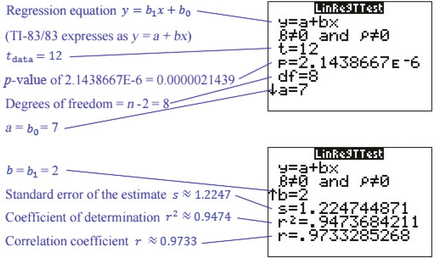 FIGURE 10 TI-83/84 regression results.Page 725
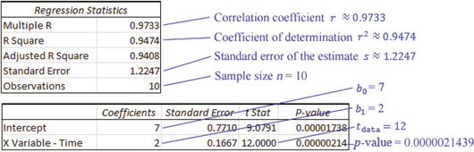 FIGURE 11 Excel regression result.
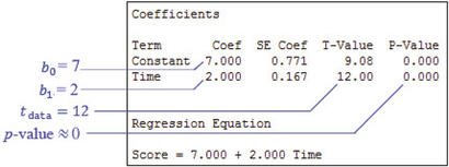 FIGURE 12 Minitab regression results.
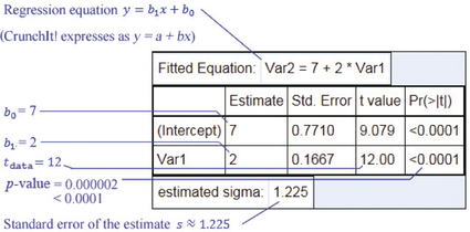 FIGURE 13 Crunchit! regression results.
Step 4 The p-value of about 0.000 is ≤ α = 0.01, so we reject H0. Evidence exists, at level of significance α = 0.01, for a linear relationship between time and score.
NOW YOU CAN DO
Exercises 19–22.
YOUR TURN#3
Recall the age and score data from the Your Turn #1 on page 717. Test, using level of significance α = 0.05, whether a linear relationship exists between age and score.
(The solution is shown in Appendix A.)
3 Confidence Interval for Slope β1
Recall that in Chapter 8 we constructed a confidence interval estimate for a population parameter, consisting of an interval of numbers that contain the parameter with a certain confidence level. Similarly, we can construct a confidence interval for the slope of the population regression equation β1.
Confidence Interval for β1
When the regression assumptions are met, a 100(1 − α)% confidence interval for β1 is given by
b1±tα/2·s√∑(x−ˉx)2
where b1 is the point estimate of the slope β1 of the population regression equation, s is the standard error of the estimate, and tα/2 has n −2 degrees of freedom.
Margin of Error E
The margin of error for a 100 (1 − α)% confidence interval for β1 is given by
E = tα/ 2· s√∑(x − ˉx)2
Thus, the confidence interval for β1 takes the form b1±E.
EXAMPLE 6 Confidence interval for the slope β1
Construct a 95% confidence interval for the slope β1 of the population regression equation for the memory-test data in Example 5.
Solution
The regression assumptions were verified in Example 5, where we found:
- b1 = 2,
- s = 1.224744871, and
- ∑(x − ˉx)2 = 54.
From the t table (Appendix Table D), we find that, for 95% confidence, tα / 2 for n − 2 = 10 − 2 = 8 degrees of freedom is tα /2 = 2.306. So, our margin of error E is
E = tα /2· s√∑(x − ˉx)2 = (2.306)(1.224744874√54) ≈ 0.3843
The 95% confidence interval for β1 is then given by
b1±E=2±0.3843=(1.6157,2.3843)
NOW YOU CAN DO
Exercises 23–30.
What Do These Numbers Mean?
- The margin of error E = 0.3843 means that, when we repeatedly take samples from this population, most of the time the sample estimate b1 will be within E = 0.3843 of the unknown value of the slope β1 of the population regression line.
- We are 95% confident that the interval (1.6157 , 2.3843) captures the slope β1 of the population regression line.
- Because β1 is the increase in memory-test score per added minute of memorization, we are 95% confident that, for each additional minute of memorization, the increase in memory-test score will lie between 1.6157 and 2.3843 points.
4 Using Confidence Intervals to Perform the t Test for the Slope β1
As in earlier sections, we may use a 100(1−α)% t confidence interval for the slope β1 to perform the t test for β1, which is a two-tailed test.
Equivalence of a Two-Tailed t Test About β1 and a t Confidence Interval for β1
- If a 100(1−α)% t confidence interval for β1 does not contain zero, then we would reject H0:β1=0 for level of significance α, and conclude that a linear relationship exists between x and y.
- If a 100(1−α)% t confidence interval for β1 does contain zero, then we would not reject H0:β1=0 for level of significance α.
EXAMPLE 7 Using confidence intervals to perform the t test for the slope β1
- Construct and interpret a 99% confidence interval for the slope β1 for the text messaging data in Table 1.
- Use the confidence interval in (a) to test whether a linear relationship exists between age and text messages, using level of significance α=0.01.
textms
Solution
- The regression assumptions were verified in Example 2. Also,
From the t table, we find that, for 99% confidence, tα/2 for n−2=10−2=8 degrees of freedom is tα/2=3.355. So, our margin of error E si
E=tα/2·s√∑(x−ˉx)2=(3.355)(2.408318916√330)≈0.4448
The 99% confidence interval for β1 is then given by
b1±E=−1.5±0.4448=(−1.9448,−1.0552)
We are 99% confident that the interval (−1.9448, −1.0552) captures the slope β1 of the population regression line. That is, we are 99% confident that, for each additional year of age, the decrease in the number of text messages lies between 1.9448 and 1.0552.
The hypotheses are
H0:β1=0 No linear relationship exists between age and text messages.
Ha:β1≠0 A linear relationship exists between age and text messages.
The confidence interval from (a) does not contain zero, so we may conclude that a linear relationship exists between age and text messages, at level of significance α=0.01.
NOW YOU CAN DO
Exercises 31–38.
| Letter | Rel. freq. in English language |
Frequency in Scrabble |
Point value in Scrabble |
Letter | Rel. freq. in English language |
Frequency in Scrabble |
Point value in Scrabble |
|---|---|---|---|---|---|---|---|
| A | 0.073 | 9 | 1 | N | 0.078 | 6 | 1 |
| B | 0.009 | 2 | 3 | O | 0.074 | 8 | 1 |
| C | 0.030 | 2 | 3 | P | 0.027 | 2 | 3 |
| D | 0.044 | 4 | 2 | Q | 0.003 | 1 | 10 |
| E | 0.130 | 12 | 1 | R | 0.077 | 6 | 1 |
| F | 0.028 | 2 | 4 | S | 0.063 | 4 | 1 |
| G | 0.016 | 3 | 2 | T | 0.093 | 6 | 1 |
| H | 0.035 | 2 | 4 | U | 0.027 | 4 | 1 |
| I | 0.074 | 9 | 1 | V | 0.013 | 2 | 4 |
| J | 0.002 | 1 | 8 | W | 0.016 | 2 | 4 |
| K | 0.003 | 1 | 5 | X | 0.005 | 1 | 8 |
| L | 0.035 | 4 | 1 | Y | 0.019 | 2 | 4 |
| M | 0.025 | 2 | 3 | Z | 0.001 | 1 | 10 |
 How Fair Is the Scoring in Scrabble?
scrabble
In this Case Study, we consider the frequency and point values of Scrabble tiles. Table 5 shows the relative frequency in the English language, the frequency (number of tiles) in Scrabble, and the point value in Scrabble.
First of all, what is the relationship between the tile frequencies in Scrabble and the letter frequencies in the English language? Figure 14 shows a scatterplot of the tile frequencies in Scrabble against the letter frequencies in the English language. A positive relationship appears to exist between the two variables. That is, as the English frequencies increase, game frequencies also tend to increase.
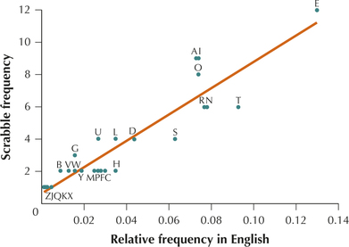
Note that the letters above the regression line occur “too frequently” in the game, whereas the letters below the line occur “not frequently enough.” Playing typical English words during a game of Scrabble would tend to leave you with a rack of letters similar to those above the regression line. Note that S is one of the letters that is rarer in the game than in the language.

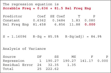
Figure 15 displays the Minitab results from a regression of the tile frequencies against the English language relative frequencies. The regression equation is
ˆy = 81.5 (relative frequency in Engilish) + 0.636
The slope is positive, which concurs with the scatterplot in Figure 14.
Next, we turn to the hypothesis test:
- H0 : β1 = 0 No linear relationship exists between Scrabble frequency and English relative frequency.
- Ha : β1 ≠ 0 A linear relationship exists between Scrabble frequency and English relative frequency.
The 0.000 in red represents the p -value for the t test. This p-value is smaller than any α, so we reject the null hypothesis that no linear relationship exists between the game frequencies and the English frequencies. Does the model fit the data well? The coefficient of determination r2 is 0.855, which is good, and the correlation coefficient r equals 0.924, which indicates that the variables are positively correlated.
But the fit really could be better. Look at the value of s , the standard error of the estimate: s ≈ 1.16 . This means that, given the English language frequency of a letter, the estimate of the tile frequency will typically differ from the actual tile frequency by more than one tile.
Next, what is the relationship between the Scrabble point values and the English relative frequencies? Figure 16 shows a scatterplot of these two variables. The first thing you might notice about this relationship is that it is not linear. Therefore, it would not be appropriate to perform linear regression on this data set.
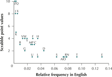
We can, nevertheless, make some descriptive remarks.
- What is a “good” Scrabble tile to pick up? In the best case, it would be a letter with high English frequency worth lots of Scrabble game points. Unfortunately, the two do not go together. The high-frequency letters such as E and T have low point values, and the high point-value letters such as Q and Z have low frequencies. But we can still make comparisons.
- Which would you rather pick up, a D or a G? It would seem that D would be preferable because it has the same point value as G with much higher English frequency.
- Which do you prefer between J and X? They are worth the same points, but X has a higher frequency in English, so it is easier to make words with it in the game. The letter H seems to have a good combination of high points and moderate frequency.