Section 9.4 Exercises
CLARIFYING THE CONCEPTS
Question 9.197
1. What assumption is required for performing the Z test that is not required for the t test? (p. 525)
9.4.1
The population standard deviation σ is known.
Question 9.198
2. What do we use to estimate the unknown population standard deviation σ? (p. 525)
PRACTICING THE TECHNIQUES
 CHECK IT OUT!
| To do | Check out | Topic |
|---|---|---|
| Exercises 3–8 | Example 18 | One-tailed t test for μ: critical value method |
| Exercises 9–14 | Example 19 | Two-tailed t test for μ: critical value method |
| Exercises 15–20 | Example 20 | One-tailed t test for μ: p-value value method |
| Exercises 21–26 | Example 21 | Two-tailed t test for μ: p-value method |
| Exercises 27–30 | Example 22 | Estimating the p-value for a t test for μ |
| Exercises 31–36 | Example 23 | Equivalence between confidence intervals and two-tailed t tests for μ |
| Exercises 37–40 | Example 24 | Interpreting software output |
For Exercises 3–14, do the following:
- State the hypotheses.
- Calculate the t critical value tcrit and state the rejection rule. Also, sketch the critical region.
- Find the test statistic tdata.
- State the conclusion and the interpretation.
Question 9.199
3. H0:μ=22 vs. Ha:μ<22, ˉx=20, s=4, n=31, α=0.05
9.4.3
(a) H0:μ=22 vs. Ha:μ<22 (b) tcrit=−1.697. Reject H0 if tdata≤−1.697.
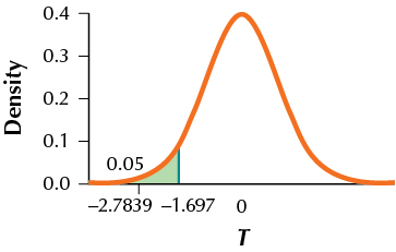
(c) tdata=−2.7839 (d) Since tdata=−2.7839 is ≤−1.697, the conclusion is reject H0. There is evidence at the 0.05 level of significance that the population mean is less than 22.
Question 9.200
4. H0:μ=3 vs. Ha:μ<3, ˉx=2, s=1, n=41, α=0.10
Question 9.201
5. H0:μ=11 vs. Ha:μ>11, ˉx=12, s=3, n=16, α=0.01, population is normal
9.4.5
(a) H0:μ=11 vs. Ha:μ>11 (b) tcrit=2.602. Reject H0 if tdata≥2.602.
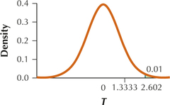
(c) tdata=1.3333 (d) Since tdata=1.3333 is not ≥2.602, the conclusion is do not reject H0. There is insufficient evidence at the 0.01 level of significance that the population mean is greater than 11.
Question 9.202
6. H0:μ=80 vs. Ha:μ>80, ˉx=82, s=5, n=9, α=0.05, population is normal
Question 9.203
7. A random sample of size 25 from a normal population yields ˉx=104 and s=10. Researchers are interested in finding whether the population mean exceeds 100, using level of significance α=0.01.
9.4.7
(a) H0:μ=100 vs. Ha:μ>100 (b) tcrit=2.492. Reject H0 if tdata≥ 2.492.
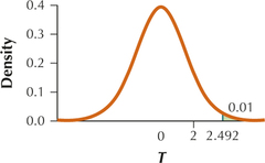
(c) tdata=2 (d) Since tdata=2 (d) is not ≥2.492, the conclusion is do not reject H0. There is insufficient evidence at the 0.01 level of significance that the population mean is greater than 100.
Question 9.204
8. A random sample of size 100 from a population with an unknown distribution yields a sample mean of −5 and a sample standard deviation of 5. Researchers are interested in finding whether the population mean is less than −4, using level of significance α=0.05.
Question 9.205
9. H0:μ=102 vs. Ha:μ≠102, ˉx=106, s=10, n=81, α=0.05
9.4.9
(a) H0:μ=102 vs. Ha:μ≠102 (b) tcrit=1.990. Reject H0 if tdata≤−1.990 or if tdata≥1.990.
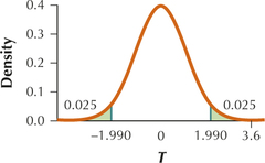
(c) tdata=3.6 (d) Since tdata=3.6 is ≥1.990, the conclusion is reject H0. There is evidence at the 0.05 level of significance that the population mean differs from 102.
Question 9.206
10. H0:μ=95 vs. Ha:μ≠95, ˉx=99, s=10, n=31, α=0.01
Question 9.207
11. H0:μ=1000 vs. Ha:μ≠1000, ˉx=975, s=100, n=25, α=0.10, population is normal
9.4.11
(a) H0:μ=1000 vs. Ha:μ≠1000 (b) tcrit=1.711. Reject H0 if tdata≤−1.711 or if tdata≥1.711.
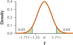
(c) tdata=−1.25 (d) Since tdata=−1.25 is not ≤−1.711 and not ≥1.711, the conclusion is do not reject H0. There is insufficient evidence at the 0.10 level of significance that the population mean differs from 1000.
Question 9.208
12. H0:μ=−10 vs. Ha:μ≠-10, ˉx=−8, s=5, n=25, α=0.05, population is normal
Question 9.209
13. A random sample of size 36 from a population with an unknown distribution yields ˉx=10 and s=3. Researchers are interested in finding whether the population mean differs from 9, using level of significance α=0.10.
9.4.13
(a) H0:μ=9 vs. Ha:μ≠9 (b) tcrit=1.690. Reject H0 if tdata≤−1.690 or if ≥1.690.
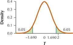
(c) tdata=2 (d) Since tdata=2 is ≥1.690, the conclusion is reject H0. There is evidence at the 0.10 level of significance that the population mean differs from 9.
Question 9.210
14. A random sample of size 16 from a normal population yields ˉx=995 and s=15. Researchers are interested in finding whether the population mean differs from 1000, using level of significance α=0.01.
For Exercises 15–26, do the following:
- State the hypotheses and the rejection rule using the p-value method.
- Calculate the test statistic tdata.
- Find the p-value. (Use technology or estimate the p-value.)
- State the conclusion and the interpretation.
Question 9.211
15. H0:μ=10 vs. Ha:μ<10, ˉx=7, s=5, n=81, α=0.01
9.4.15
(a) H0:μ=10 vs. Ha:μ<10. Reject H0 if the p-value≤α=0.01 (b) tdata=−5.4 (c) 0 (d) Since the p-value=0 is ≤α=0.01, the conclusion is reject H0. There is evidence at the 0.01 level of significance that the population mean is less than 10.
Question 9.212
16. H0:μ=50 vs. Ha:μ<50, ˉx=42, s=8, n=41, α=0.05
Question 9.213
17. H0:μ=100 vs. Ha:μ>100, ˉx=120, s=50, n=25, α=0.10, population is normal
9.4.17
(a) H0:μ=100 vs. Ha:μ>100. Reject H0 if the p-value≤α=0.10 (b) tdata=2 (c) 0.0285 (d) Since the p-value=0.0285 is ≤α=0.10, the conclusion is reject H0. There is evidence at the 0.10 level of significance that the population mean is greater than 100.
Question 9.214
18. H0:μ=3.0 vs. Ha:μ>3.0, ˉx=3.2, s=0.5, n=25, α=0.05, population is normal
Question 9.215
19. A random sample of size 400 from a population with an unknown distribution yields a sample mean of 230 and a sample standard deviation of 5. Researchers are interested in finding whether the population mean is greater than 200, using level of significance α=0.05.
9.4.19
(a) H0:μ=200 vs. Ha:μ>200. Reject H0 if the p-value≤α=0.05 (b) tdata=120 (c) 0 (d) Since the p-value=0 is ≤α=0.05, the conclusion is reject H0. There is evidence at the 0.05 level of significance that the population mean is greater than 200.
Question 9.216
20. A random sample of size 100 from a population with an unknown distribution yields ˉx=27 and s=10. Researchers are interested in finding whether the population mean is less than 28, using level of significance α=0.05.
Question 9.217
21. H0:μ=25 vs. Ha:μ≠25, ˉx=25, s=1, n=31, α=0.01
9.4.21
(a) H0:μ=25 vs. Ha:μ≠25. Reject H0 if the p-value≤α=0.01 (b) tdata=0 (c) 1 (d) Since the p-value=1 is not ≤α=0.01, the conclusion is do not reject H0. There is insufficient evidence at the 0.01 level of significance that the population mean differs from 25.
Question 9.218
22. H0:μ=98.6 vs. Ha:μ≠98.6, ˉx=99, s=10, n=81, α=0.05
Question 9.219
23. H0:μ=3.14 vs. Ha:μ≠3.14, ˉx=3.17, s=0.5, n=9, α=0.10, population is normal
9.4.23
(a) H0:μ=3.14 vs. Ha:μ≠3.14. Reject H0 if the p-value≤α=0.10 (b) tdata=0.18 (c) 0.8616 (d) Since the p-value=0.8616 is not ≤α=0.10, the conclusion is do not reject H0. There is insufficient evidence at the 0.10 level of significance that the population mean differs from 3.14.
Question 9.220
24. H0:μ=2.72 vs. Ha:μ≠2.72, ˉx=2.57, s=0.1, n=25, α=0.05, population is normal
Question 9.221
25. A random sample of size 9 from a normal population yields ˉx=1 and s=0.5. Researchers are interested in finding whether the population mean differs from 0, using level of significance α=0.05.
9.4.25
(a) H0:μ=0 vs. Ha:μ≠0. Reject H0 if the p-value≤α=0.05 (b) tdata=6 (c) 0.0003 (d) Since the p-value=0.0003 is ≤α=0.05, the conclusion is reject H0. There is evidence at the 0.05 level of significance that the population mean differs from 0.
Question 9.222
26. A random sample of size 16 from a normal population yields ˉx=2.2 and s=0.3. Researchers are interested in finding whether the population mean differs from 2.0, using level of significance α=0.01.
For Exercises 27–30, use the t table to estimate the p-value for the hypothesis tests in the indicated exercises.
Question 9.223
27. Exercise 3
9.4.27
p-value<0.005
Question 9.224
28. Exercise 4
Question 9.225
29. Exercise 9
9.4.29
p-value<0.01
Question 9.226
30. Exercise 10
For Exercises 31–36, 100(1-α)%t confidence interval is given. Use the confidence interval to test, using level of significance α, whether μ differs from each of the indicated hypothesized values.
Question 9.227
31. A 95% t confidence interval for μ is (1, 4).
Hypothesized values μ0 are
- 0
- 2
- 5
9.4.31
| Value of μ0 |
Form of hypothesis test, with α=0.05 |
Where μ0 lies in relation to 95% confidence interval (1, 4) |
Conclusion of hypothesis test |
|
|---|---|---|---|---|
| (a) | 0 | H0:μ=0 vs.Ha:μ≠0 | Outside | Reject H0 |
| (b) | 2 | H0:μ=2 vs.Ha:μ≠2 | Inside | Do not reject H0 |
| (c) | 5 | H0:μ=5 vs.Ha:μ≠5 | Outside | Reject H0 |
Question 9.228
32. A 99% t confidence interval for μ is (57, 58).
Hypothesized values μ0 are
- 55.5
- 59.5
- 57.5
Question 9.229
33. A 90% t confidence interval for μ is (−20, −10).
Hypothesized values μ0 are
- −21
- −5
- −12
9.4.33
| Value of μ0 |
Form of hypothesis test, with α=0.10 |
Where μ0 lies in relation to 90% confidence interval (–20, −10) |
Conclusion of hypothesis test | |
|---|---|---|---|---|
| (a) | –21 | H0:μ=−21 vs.Ha:μ≠−21 | Outside | Reject H0 |
| (b) | –5 | H0:μ=−5 vs.Ha:μ≠−5 | Outside | Reject H0 |
| (c) | –12 | H0:μ=−12 vs.Ha:μ≠−12 | Inside | Do not reject H0 |
Question 9.230
34. A 95% t confidence interval for μ is (2010, 2015).
Hypothesized values μ0 are
- 2012
- 2007
- 2014
Question 9.231
35. A 95% t confidence interval for μ is (−1, 1).
Hypothesized values μ0 are
- 1.5
- −1.5
- 0
9.4.35
| Value of μ0 |
Form of hypothesis test, with α=0.05 |
Where μ0 lies in relation to 95% confidence interval (−1, 1) |
Conclusion of hypothesis test |
|
|---|---|---|---|---|
| (a) | 1.5 | H0:μ=1.5 vs.Hα:μ≠1.5 | Outside | Reject H0 |
| (b) | –1.5 | H0:μ=−1.5 vs.Hα:μ≠−1.5 | Outside | Reject H0 |
| (c) | 0 | H0:μ=0 vs.Hα:μ≠0 | Inside | Do not reject H0 |
Question 9.232
36. A 95% t confidence interval for μ is (19,570, 20,105).
Hypothesized values μ0 are
- 20,000
- 21,000
- 19,571
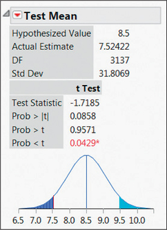
For Exercises 37–40, software output from a t test for μ is provided. For each, examine the indicated software output, and provide the following steps:
- Step 1 State the hypotheses and the rejection rule.
- Step 2 Find Zdata.
- Step 3 Find the p-value.
- Step 4 State the conclusion and interpretation.
Use level of significance α=0.05 for each hypothesis test.
Question 9.233
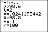
37. TI-83/84 output
9.4.37
Step 1 H0:μ=98.6 vs. Ha:μ>98.6
We will reject H0 if the p-value≤α=0.05.
Step 2 tdata=2
Step 3 p-value=0.0241198442
Step 4 The p-value=0.0241198442 is ≤0.05. Therefore we reject H0. There is evidence at level of significance α=0.05 that the population mean is greater than 98.6.
Question 9.234
38. Minitab output

Question 9.235
39. SPSS output

9.4.39
Step 1 H0:μ=20 vs. Ha:μ≠20
We will reject H0 if the p-value≤α=0.05.
Step 2 tdata=2.308
Step 3 p-value=0.021
Step 4 The p-value=0.021 is ≤0.05. Therefore we reject H0. There is evidence at level of significance α=0.05 that the population mean is not equal to 20.
Question 9.236
40. JMP output: Choose the left-tailed test.
APPLYING THE CONCEPTS
Question 9.237
41. Health Care Costs. The U.S. Agency for Healthcare Research and Quality (www.ahrq.gov) reports that, in 2010, the mean cost of a stay in the hospital for American women ages 18–44 was $15,200. A recent random sample of 400 hospital stays of women ages 18–44 showed a mean cost of $16,000, with a standard deviation of $5000. Test whether the population mean cost has increased since 2010, using level of significance α=0.05.
9.4.41
Critical-value method: H0:μ=15,200 vs. Ha:μ>15,200. tcrit=1.660. Reject H0 if tdata≥1.660. tdata=3.2. Since tdata=3.2 is ≥1.660, the conclusion is reject H0. There is evidence at the 0.05 level of significance that the population mean cost of a stay in the hospital for women aged 18–44 is greater than $15,200. Therefore we can conclude at level of significance 0.05 that the population mean cost of a stay in the hospital for American women aged 18–24 has increased since 2010. p-value method: H0:μ=15,200 vs. Ha:μ>15,200. Reject H0if the p-value≤α=0.05. tdata=3.2. p-value=0.0007. Since the p-value=0.0007 is ≤α=0.05, the conclusion is reject H0. There is evidence at the 0.05 level of significance that the population mean cost of a stay in the hospital for women aged 18–44 is greater than $15,200. Therefore we can conclude at level of significance 0.05 that the population mean cost of a stay in the hospital for American women aged 18-24 has increased since 2010.
Question 9.238
42. iPhone Apps. According to a 2010 Nielsen survey,9 the mean number of apps downloaded by iPhone users is 40. Suppose a recent sample of 36 iPhone users downloaded an average of 45 apps, with a standard deviation of 24. Test whether the population mean number of apps is greater than 40, using level of significance α=0.10.
Question 9.239
43. Facebook Friends. According to Facebook.com, the mean number of Facebook friends is 130. Suppose a sample of 100 Facebook users has a mean number of 110 Facebook friends, with a standard deviation of 50. Test whether the population mean number of Facebook friends is less than the reported 130, using level of significance α=0.05.
9.4.43
Critical-value method: H0:μ=130 vs. Ha:μ<130. tcrit=−1.662. Reject H0 if tdata≤−1.662. tdata=−4. Since tdata=−4 is ≤−1.662, the conclusion is reject H0. There is evidence at the 0.05 level of significance that the population mean number of Facebook friends is less than 130. p-value method: H0:μ=130 vs. Ha:μ<130. Reject H0 if p-value≤α=0.05. tdata=−4. p-value=0. Since the p-value=0 is ≤α=0.05, the conclusion is reject H0. There is evidence at the 0.05 level of significance that the population mean number of Facebook friends is less than 130.
Question 9.240
44. Small Business Employees. The U.S. Census Bureau reports that the average number of employees in a small business is 16.1. Suppose a sample of 49 small businesses showed a mean of 15 employees, with a standard deviation of 25. Test whether the population mean number of employees in a small business is different from the reported 16.1, using level of significance α=0.01.
Internet Response Times. Use the following information for Exercises 45 and 46: The Web site www.internettrafficreport.com monitors Internet traffic worldwide and reports on the response times of randomly selected servers.
Question 9.241
45. On June 6, 2011, the Web site reported the following response times to Asia, in milliseconds:
| 165 | 175 | 2221 | 872 | 311 | 127 | 195 | 1801 | 769 | 225 | 261 | 249 | 421 |
We want to test whether the population mean response time is slower than 180 milliseconds, using a t test and level of significance α=0.05. A boxplot of the data is provided.

(Hint: The boxplot is right-skewed and the normal distribution is symmetric.) Can we proceed with the t test? Explain.
9.4.45
No. The distribution of the variable is not normal and the sample size is less than 30.
Question 9.242
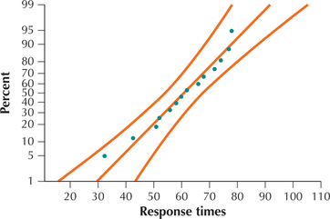
46. On June 6, 2011, the Web site reported the following response times to Asia, in milliseconds:
| 61 | 32 | 50 | 73 | 51 | 42 | 55 | 65 | 59 | 57 | 76 | 77 | 67 | 71 |
The normal probability plot of the data is also shown. We want to perform a t test.
- Are the conditions for performing the t test satisfied? Explain how you know.
- Test, using level of significance α=0.05, whether the population mean response time is less than 60 milliseconds.
- Explain why we can't use a Z test for this problem.
Deepwater Horizon Cleanup Costs. The following table represents the amount of money disbursed by BP to a random sample of six Florida counties, for cleanup of the Deepwater Horizon oil spill, in millions of dollars.10 Use the following information for Exercises 47–49.
| County | Cleanup costs ($ millions) |
|---|---|
| Broward | 0.85 |
| Escambia | 0.70 |
| Franklin | 0.50 |
| Pinellas | 1.15 |
| Santa Rosa | 0.50 |
| Walton | 1.35 |
Question 9.243
deepwaterclean
47. The normality of the data was confirmed in the Section 8.1 exercises. Test, at level of significance α=0.10, whether the population mean amount of cleanup money exceeds $500,000.
9.4.47
Step 1 H0:μ=500,000 vs. Ha:μ>500,000 We will reject H0 if the p-value≤α=0.10.
Step 2 tdata=2.4018
Step 3 p-value=0.0307414454
Step 4 The p-value=0.0307414454 is ≤0.10. Therefore we reject H0. There is evidence at level of significance α=0.10 that the population mean amount of cleanup money is greater than $500,000.
Question 9.244
deepwaterclean
48. Answer the following:
- Repeat your test from Exercise 47, this time using level of significance α=0.01.
- How do you think we should resolve the apparent contradiction in Exercise 47 and part (a) of this exercise?
- Assess the strength of the evidence against the null hypothesis. Does this change depending on which level of α you use?
Question 9.245
deepwaterclean
 49.What if we changed μ0 to some larger value (though still smaller than ˉx)? Otherwise, everything else remains unchanged. Describe how this change would affect the following, if at all:
- tdata
- tcrit
- The p-value
- The conclusion from Exercise 47
- The conclusion from Exercise 48(a)
- The strength of the evidence against the null hypothesis
9.4.49
(a) Decrease (b) Stay the same (c) Increase (d) Depends on new value of μ0 (e) Stay the same (f) Depends on new value of μ0
Question 9.246
wiisales
50. Wii Game Sales. The following table represents the number of units sold in the United States for the week ending March 26, 2011, for a random sample of eight Wii games.11 The normality of the data was confirmed in the Section 8.1 exercises.
- Construct and interpret a 95% t interval for the population mean number of units sold. (See Section 8.2.)
- Use your confidence interval to test, using level of significance α=0.05, whether μ differs from the following values:
- 30,000 units
- 31,000 units
- 0 units
- 79,000 units
| Game | Units (1000s) |
Game | Units (1000s) |
|---|---|---|---|
| Wii Sports Resort | 65 | Zumba Fitness | 56 |
| Super Mario All Stars | 40 | Wii Fit Plus | 36 |
| Just Dance 2 | 74 | Michael Jackson | 42 |
| New Super Mario Bros. |
16 | Lego Star Wars | 110 |
Question 9.247
georgiarain
51. A Rainy Month in Georgia? The following table represents the total rainfall (in inches) for the month of February 2011 for a random sample of 10 locations in Georgia.12 The normality was checked in the Section 8.1 exercises. Test whether the population mean amount of rainfall differs from 4 inches, using level of significance α=0.10.
| Location | Rainfall (inches) |
Location | Rainfall (inches) |
|---|---|---|---|
| Athens | 4.72 | Atlanta | 4.25 |
| Augusta | 4.31 | Cartersville | 3.03 |
| Dekalb | 2.96 | Fulton | 4.36 |
| Gainesville | 4.06 | Lafayette | 3.75 |
| Marietta | 3.20 | Rome | 3.26 |
9.4.51
Step 1 H0:μ=4 vs. Ha:μ≠4 We will reject H0 if the p-value≤α=0.10.
Step 2 tdata=−1.044
Step 3 p-value=0.3237340082
Step 4 The p-value=0.3237340082 is not ≤0.10. Therefore we do not reject H0. There is insufficient evidence at level of significance α=0.10 that the population mean amount of rainfall differs from 4 inches.
Question 9.248
electricmiles
52. Electric Cars. The accompanying table shows the miles-per-gallon equivalent (MPGe) for five electric cars, as reported by www.hybridcars.com in 2014. Assume the data are drawn from a normal distribution. Test whether the population mean mileage is greater than 90 MPGe, using level of significance α=0.10.
| Electric Vehicle | Mileage (MPGe) |
|---|---|
| Tesla Model S | 89 |
| Nissan Leaf | 99 |
| Ford Focus | 105 |
| Mitsubishi i-MiEV | 112 |
| Chevrolet Spark | 119 |
BRINGING IT ALL TOGETHER
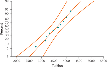
Community College Tuition. Use the following information for Exercises 53–63. The College Board reported that the mean tuition and fees at community colleges nationwide for the 2013–2014 academic year was $3264. Data were gathered on the total tuition and fees for a random sample of 10 community colleges in 2015. The normal probability plot is shown here.
Question 9.249
53. Is it appropriate to apply the t test for the mean? Why or why not?
9.4.53
Yes. The normal probability plot indicates acceptable normality.
Question 9.250
54. Find the t critical value for a right-tailed hypothesis test using level of significance α=0.05.
Question 9.251
55. For the sample of 10 community colleges, the sample mean tuition and fees was $3541 with a sample standard deviation of $438. Test whether the population mean tuition and fees have increased using level of significance α=0.05.
9.4.55
Step 1 H0:μ=3264 vs. Ha:μ>3264
Step 2 tcrit=1.833 Reject H0 if tdata≥1.833.
Step 3t=2.000
Step 4 tdata=2.000 is ≥1.833. Therefore we reject H0. There is evidence at level of significance α=0.05 that the population mean tuition and fees for community colleges has increased from the previous level of $3264.
Question 9.252
56. Estimate the p-value for the hypothesis test in the previous exercise.
Question 9.253
57. Assess the strength of evidence against the null hypothesis.
9.4.57
There is solid evidence against the null hypothesis that the population mean is $3264.
Question 9.254
58. A 95% confidence interval for the population mean tuition and fees is given by lower bound = $3227, upper bound = $3854. Use this confidence interval to test, at level of significance α=0.05, whether μ differs from the following values.
- $4000
- $3500
- $3264
Question 9.255
59. A data analyst, in attempting to use technology to test whether the population mean tuition and fees have increased, obtained the following Minitab output. However, it appears that the analyst asked for the wrong hypothesis test. How can you tell?

9.4.59
The line “Test of μ=3264 vs. ≠3264.”
Question 9.256
60. How can we use the p-value on the Minitab printout to find the p-value needed for the right-tailed hypothesis test we performed in Exercise 55?
Question 9.257
61. Suppose, when we did Exercise 55, we also asked for the wrong hypothesis test, and obtained this Minitab output. For level of significance α=0.05, what would have been our conclusion in that case? Why would this have been in error? What are some of the possible consequences of making an error of this sort?
9.4.61
Do not reject H0. Fees have increased. Answers will vary.
Question 9.258
62. Based on your experiences in these exercises, write a sentence about the importance of understanding the statistics behind the “point and click” power of statistical software.
Question 9.259
63. Challenge Exercise. Note that we have concluded that there is insufficient evidence that the population mean cost has changed, but evidence exists that the population mean cost has increased. How can the mean cost have increased without changing? Explain what is going on here, in terms of either critical regions or p-values.
9.4.63
Since the p-value for the two-tailed test is twice the p-value for the one-tailed test, it is possible to conclude that there is insufficient evidence that the population mean cost has changed, but there is evidence that the population mean cost has increased if α is between the two p-values.
WORKING WITH LARGE DATA SETS
New York Towns. Work with the New York data set for Exercises 64 and 65.
Question 9.260
newyork
64. Use technology to find the summary statistics for the variable tot_pop, which lists the population for each of the towns and cities in New York with at least 1000 people.
Question 9.261
newyork
65. Suppose we are using the data in this data set as a sample of the population of all the towns and cities in the northeastern United States with at least 1000 people. Use technology to test at level of significance α=0.05 whether the population mean of these towns differs from 50,000.
9.4.65

WORKING WITH LARGE DATA SETS
Fast Food versus Full Service Restaurants. Open the data set, Restaurants. Here, we will look at the variable FFR per 1000, which refers to the number of fast food restaurants per 1000 residents of the county. For example, a value of 0.6 would mean that there are 0.6 fast food restaurants per 1000 residents in the county. We will perform a hypothesis test for the population mean FFR per 1000. We will then see whether this hypothesis test made the correct decision. Use technology to do the following:
Question 9.262
restaurants
66. Obtain a random sample of size 100 from the data set.
Question 9.263
restaurants
67. Using your sample, test whether the population mean number of fast food restaurants per 1000 residents differs from 0.4, using level of significance α=0.05.
Question 9.264
restaurants
68. Find the actual value of the population mean number of fast food restaurants per county. Did your hypothesis test in Exercise 67 make the right decision? Explain.
WORKING WITH LARGE DATA SETS
 Chapter 9 Case Study: Clothing Store Sales. Open the Chapter 9 Case Study data set, Clothing Store. Retail stores want you to come back again and again, with a short amount of time between purchases. The Clothing Store data set tracks the number of days since the last purchase for each customer. The marketing manager wants to make sure that the mean number of days since the last purchase is less than 150 days. Use technology to do the following:
Question 9.265
clothingstore
69. Obtain a random sample of size 100 from the data set.
Question 9.266
clothingstore
70. Using your sample, test whether the population mean number of days since the last purchase is less than 150, using level of significance α=0.05.