12.2 Limits and ContinuityPrinted Page 819
819
In Chapters 1 and 2, we saw the importance of the limit of a function of one variable in determining continuity and defining and finding the derivative. Limits of functions of several variables play a similar role.
1 Define the Limit of a Function of Several VariablesPrinted Page 819
We begin by reviewing the definition of a limit (Chapter 1, pp. 76 and 132).
Let f be a function of one variable defined everywhere in an open interval containing c, except possibly at c. Then the limit of f(x) as x approaches c is L, written \bbox[5px, border:1px solid black, #F9F7ED]{\bbox[#FAF8ED,5pt] { \lim\limits_{x\rightarrow c}f(x)=L }}
if for any number \varepsilon >0, there is a number \delta > 0, so that \bbox[5px, border:1px solid black, #F9F7ED]{\bbox[#FAF8ED,5pt] { \hbox{whenever }\ 0<\left\vert x-c\right\vert <\delta \qquad \hbox{then}\qquad \vert f(x)-L\vert <\varepsilon }}
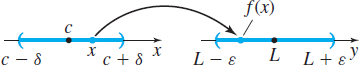
In this definition, the phrase “whenever 0<\left\vert x-c\right\vert <\delta ” means “for all x, x \ne c, within a distance \delta of c,” and “\left\vert f(x) -L\right\vert <\varepsilon ” means “the corresponding value of f is within a distance \varepsilon of L.” See Figure 18.
The definition of a limit for functions of two or more variables is similar, but requires additional terminology.
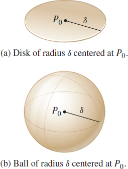
DEFINITION \delta -Neighborhood; Disk; Ball
Let P_{0} be a point in the plane or in space. A \delta -neighborhood of P_{0} consists of all the points P that lie within a distance \delta of P_{0}. That is, a \delta -neighborhood consists of all points P for which d(P, P_{0})<\delta , where d( P,P_{0}) is the distance from P to P_{0}.
- In the plane, a \delta -neighborhood of P_{0} is called a disk of radius \delta centered at P_{0}.
- In space, a \delta -neighborhood of P_{0} is called a ball of radius \delta centered at P_{0}.
See Figure 19.
With these definitions, we are ready to define the limit of a function of several variables.
NOTE
On a real line, a \delta-neighborhood of a number P_{0} is an open interval with P_{0} as midpoint.
DEFINITION Limit of a Function of Two Variables
Let f be a function of two variables defined at each point in some disk centered at (x_{0},\,y_{0}), except possibly at (x_{0},y_{0}). Then the limit of f(x,y) as (x,y) approaches (x_{0},y_{0}) is L if, for any given number \varepsilon >0, there is a number \delta >0, so that \bbox[5px, border:1px solid black, #F9F7ED]{\bbox[#FAF8ED,5pt] { \hbox{whenever }\ 0<\sqrt{(x-x_{0})^{2}+(y-y_{0})^{2}}<\delta \qquad \hbox{then} \qquad \vert f(x,y) -L\vert <\varepsilon }}
Then we say, “The limit exists”, and write \bbox[5px, border:1px solid black, #F9F7ED]{\bbox[#FAF8ED,5pt] { \lim\limits_{(x, y)\rightarrow (x_{0}, y_{0})}f(x,y)=L }}
820
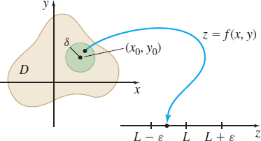


Figure 20 illustrates the definition.
DEFINITION Limit of a Function of Three Variables
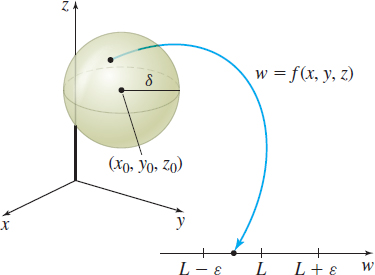
Let f be a function of three variables defined at each point in some ball centered at (x_{0},y_{0},z_{0}), except possibly at (x_{0},y_{0},z_{0}). Then the limit of f(x,y,z) as (x,y,z) approaches (x_{0},y_{0},z_{0}) is L if, for any given number \varepsilon >0, there is a number \delta >0, so that \bbox[5px, border:1px solid black, #F9F7ED]{\bbox[#FAF8ED,5pt]{ \hbox{whenever }\ 0<\sqrt{(x-x_{0})^{2}+(y-y_{0})^{2}+(z-z_{0})^{2}} <\delta \quad \hbox{then}\ \vert f(x,y,z) -L\vert <\varepsilon }}
Then we say, “The limit exists”, and write \bbox[5px, border:1px solid black, #F9F7ED]{\bbox[#FAF8ED,5pt]{ \lim\limits_{(x, y, z)\rightarrow (x_{0}, y_{0}, z_{0})}f(x,y,z)=L }}
The definition states that if you decide how close you want f to be to L, that is, if you choose \varepsilon , you can find a number \delta so that whenever the point (x,y,z) is within a distance \delta of ( x_{0},y_{0},z_{0}) , then f is within a distance \varepsilon of L. See Figure 21.
Notice the similarity of the definitions for the limit of a function of one variable, two variables, and three variables. In fact, limits of functions of more than three variables are defined similarly, as follows. Suppose f(P) is a function of one or more variables defined at each point P in some neighborhood of P_{0}, except possibly at P_{0}. Then \bbox[5px, border:1px solid black, #F9F7ED]{\bbox[#FAF8ED,5pt]{ \lim\limits_{P\rightarrow P_{0}}f(P)=L }}
if, for any given number \varepsilon >0, there is a number \delta >0, so that \bbox[5px, border:1px solid black, #F9F7ED]{\bbox[#FAF8ED,5pt]{ \hbox{whenever}\ 0<d(P, P_{0})<\delta \qquad \hbox{then}\qquad \left\vert f(P)-L\right\vert <\varepsilon }}
2 Find a Limit Using Properties of LimitsPrinted Page 821
821
The algebra of limits for functions of one variable extends to that for functions of several variables. We state the algebraic properties of limits of functions of two variables without proof. These properties are also true for functions of three or more variables.
THEOREM Algebraic Properties of Limits (Two Variables)
Let f and g be functions of two variables for which \lim_{(x, y)\rightarrow (x_{0}, y_{0})}f(x,y)=L\qquad \hbox{and}\qquad \lim_{(x, y)\rightarrow (x_{0}, y_{0})}g(x,y)=M
where L and M are two real numbers.
- Limit of a sum: \bbox[5px, border:1px solid black, #F9F7ED]{\bbox[#FAF8ED,5pt]{ \begin{eqnarray*} \lim\limits_{(x, y)\rightarrow (x_{0}, y_{0})}[f(x,y)+g(x,y)]&=&\lim\limits_{(x, y)\rightarrow (x_{0}, y_{0})}f(x,y) +\lim\limits_{(x, y)\rightarrow (x_{0}, y_{0})}g(x,y)\\ &=&L+M \end{eqnarray*}}}
- Limit of a difference: \bbox[5px, border:1px solid black, #F9F7ED]{\bbox[#FAF8ED,5pt] { \begin{eqnarray*} \lim\limits_{(x, y)\rightarrow (x_{0}, y_{0})}[f(x,y)-g(x,y)]&=&\lim\limits_{(x, y)\rightarrow (x_{0}, y_{0})}f(x,y) -\lim\limits_{(x, y)\rightarrow (x_{0}, y_{0})}g(x,y)\\ &=&L-M \end{eqnarray*}}}
- Limit of a constant times a function: If k is any real number, then \bbox[5px, border:1px solid black, #F9F7ED]{\bbox[#FAF8ED,5pt]{ \begin{eqnarray*} \lim\limits_{(x, y)\rightarrow (x_{0}, y_{0})}[k\,f(x,y)]=k\left[ \lim\limits_{(x, y)\rightarrow (x_{0}, y_{0})}f(x,y)\right] =kL \end{eqnarray*}}}
- Limit of a product: \bbox[5px, border:1px solid black, #F9F7ED]{\bbox[#FAF8ED,5pt]{ \begin{eqnarray*} \lim\limits_{(x, y)\rightarrow (x_{0}, y_{0})}[f(x,y)g(x,y)]&=&\left[ \lim\limits_{(x, y)\rightarrow (x_{0}, y_{0})}f(x,y)\right]\; \left[ \lim\limits_{(x, y)\rightarrow (x_{0}, y_{0})}g(x,y)\right]\\[4pt] &=&LM \end{eqnarray*}}}
- Limit of a quotient: If \lim\limits_{(x, y)\rightarrow (x_{0}, y_{0})}g(x,y)=M\neq 0, \bbox[5px, border:1px solid black, #F9F7ED]{\bbox[#FAF8ED,5pt]{ \lim\limits_{(x, y)\rightarrow (x_{0}, y_{0})}\dfrac{f(x,y)}{g(x,y) }=\dfrac{ \lim\limits_{(x, y)\rightarrow (x_{0}, y_{0})}f(x,y)}{\lim\limits_{(x, y) \rightarrow (x_{0}, y_{0})}g(x,y)}=\dfrac{L}{M} }}
- Limit of a constant: If c is a constant, \bbox[5px, border:1px solid black, #F9F7ED]{\bbox[#FAF8ED,5pt]{ \lim\limits_{(x, y)\rightarrow (x_{0}, y_{0})}c=c }}
- Limit of a function of a single variable: If f(x,y) =h(x) , then \bbox[5px, border:1px solid black, #F9F7ED]{\bbox[#FAF8ED,5pt]{ \lim\limits_{(x, y)\rightarrow (x_{0}, y_{0})}f(x,y)=\lim\limits_{x\rightarrow x_{0}}h(x) }}
If f(x,y) =g(y) , then \bbox[5px, border:1px solid black, #F9F7ED]{\bbox[#FAF8ED,5pt]{ \lim\limits_{(x, y)\rightarrow (x_{0}, y_{0})}f(x,y)=\lim\limits_{y\rightarrow y_{0}}g(y) }}
822
EXAMPLE 1Using Properties of Limits to Find a Limit
Find each limit:
- (a) \lim\limits_{(x, y)\rightarrow (1, 2)}(3x^{2}+2xy+y^{2})
- (b) \lim\limits_{(x, y)\rightarrow (1, 2)}\dfrac{xy}{x^{2}+y^{2}}
- (c) \lim\limits_{(x, y)\rightarrow (3, -1)}\dfrac{x^{2}+2xy-3y^{2}}{ x^{2}+9y^{2}}
Solution (a) \begin{eqnarray*} \lim_{(x, y)\rightarrow (1, 2)}(3x^{2}+2xy+y^{2})& =&\lim_{(x, y)\rightarrow (1, 2)}( 3x^{2}) +\lim_{(x, y)\rightarrow (1, 2)}( 2xy) +\lim_{(x, y)\rightarrow (1, 2)}y^{2} \\[8pt] & =&3\lim_{x\rightarrow 1}x^{2}+\Big( \lim_{(x, y)\rightarrow (1, 2)}( 2x) \Big) \Big( \lim_{(x, y)\rightarrow (1, 2)}y\Big) +\lim_{y\rightarrow 2}y^{2} \\[8pt] &=& 3+2\Big( \lim_{x\rightarrow 1}x\Big) \Big( \lim_{y\rightarrow 2}y\Big) +4=3+2\cdot 1\cdot 2+4=11 \end{eqnarray*}
(b) Since \lim\limits_{(x, y)\rightarrow (1, 2)} (x^2+y^2) = \lim\limits_{x\rightarrow 1} x^2 + \lim\limits_{y\rightarrow 2} y^2 =5\neq 0, we use the limit of a quotient: \begin{eqnarray*} \lim_{(x, y)\rightarrow (1, 2)}\frac{xy}{x^{2}+y^{2}} &=&\frac{ \lim\limits_{(x, y)\rightarrow (1, 2)}(xy) }{\lim\limits_{(x, y) \rightarrow (1, 2)}(x^{2}+y^{2})} =\frac{\Big( \lim\limits_{x\rightarrow 1}x\Big) \Big( \lim\limits_{y\rightarrow 2}y\Big) }{\lim\limits_{x\rightarrow 1}x^{2}+\lim\limits_{y\rightarrow 2}y^{2}}=\frac{1\cdot 2}{1+4}=\frac{2}{5} \end{eqnarray*}
(c) Look at the denominator. Since \lim\limits_{(x, y) \rightarrow (3,-1)}( x^{2}+9y^{2}) =18, we can use the limit of a quotient property. Then \begin{eqnarray*} \lim\limits_{(x, y)\rightarrow (3,-1)}\dfrac{x^{2}+2xy-3y^{2}}{x^{2}+9y^{2}} &=&\dfrac{\lim\limits_{(x, y)\rightarrow (3,-1)}(x^{2} + 2xy - 3y^{2}) }{\lim\limits_{(x, y)\rightarrow (3,-1)}(x^{2} + 9y^{2}) }\\[8pt] &=&\frac{\lim\limits_{x\rightarrow 3}x^{2} + 2\Big( \lim\limits_{x\rightarrow 3}x\Big) \Big( \lim\limits_{y\rightarrow -1}y\Big) - 3 \lim\limits_{y\rightarrow -1}y^{2}}{18}\\[8pt] &=&\dfrac{9 + 2(3)(-1) - 3(1)}{18}=0 \end{eqnarray*}
NOW WORK
3 Examine When Limits ExistPrinted Page 822
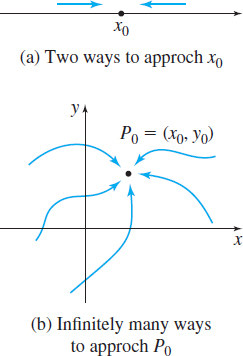
The limit of a function f of single variable exists only if the left-hand limit equals the right-hand limit. That is, \lim\limits_{x\rightarrow c}f(x) exists if the limit is the same no matter how the number c is approached. For a single variable, there are only two ways to approach c: from the left or from the right. See Figure 22(a). When z=f(x,y) is a function of two variables, however, there are infinitely many ways to approach a point P_{0}, namely along any curve that passes through P_{0}. See Figure 22(b). So, for \lim\limits_{(x,y) \rightarrow ( x_{0},y_{0}) }f(x,y) to exist, it is necessary that the same limit be obtained no matter what curve C containing P_{0} is used. Put another way, if two different curves that contain (x_{0},y_{0}) result in different limits, then \lim\limits_{(x,y) \rightarrow (x_{0},y_{0}) }f(x,y) does not exist.
823
THEOREM
If \lim\limits_{P\rightarrow P_{0}}f(P) is computed along two different curves containing P_{0} and if two different answers are obtained, then \lim\limits_{P\rightarrow P_{0}}f(P) does not exist.
EXAMPLE 2Showing That a Limit Does Not Exist
Show that \lim\limits_{(x, y)\rightarrow (0, 0)}\dfrac{xy}{ x^{2}+y^{2}} does not exist.
Solution Look at the denominator. Since \lim\limits_{(x, y) \rightarrow (0, 0)}( x^{2}+y^{2}) =0, we cannot use the limit of a quotient to investigate the limit. We investigate the limit using two curves that contain (0,0), say, y=2x and y=-x.
First we investigate the limit using the line y=2x. Then \begin{equation*} {\rm Using}\; y=2x: \quad \lim\limits_{(x, y)\rightarrow (0, 0)}\dfrac{x\left( 2x\right) }{x^{2}+\left( 2x\right) ^{2}}=\lim\limits_{x\rightarrow 0}\dfrac{ 2x^{2}}{x^{2}+4x^{2}}=\lim\limits_{x\rightarrow 0}\dfrac{2x^{2}}{5x^{2}}= \dfrac{2}{5} \end{equation*}
Now we investigate the limit using the line y=-x. \begin{equation*} {\rm Using}\; y=-x: \quad \lim\limits_{(x, y)\rightarrow (0, 0)}\dfrac{x\left( -x\right) }{x^{2}+\left( -x\right) ^{2}}=\lim\limits_{x\rightarrow 0}\dfrac{ -x^{2}}{x^{2}+x^{2}}=\lim\limits_{x\rightarrow 0}\dfrac{-x^{2}}{2x^{2}}=- \dfrac{1}{2} \end{equation*}
Since two different answers are obtained, the limit does not exist.
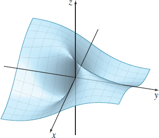
Figure 23 shows the graph of f(x,y) =\dfrac{xy}{x^{2}+y^{2}}.
NOW WORK
EXAMPLE 3Showing That a Limit Does Not Exist
Show that \lim\limits_{(x, y)\rightarrow (0, 0)}\dfrac{x^{2}y}{x^{4}+y^{2}} does not exist.
Solution We investigate the limit using curves that contain (0,0). Based on our experience with the function in Example 2, we can simultaneously test all nonvertical lines that contain (0,0) by using y=mx . Then \begin{equation*} {\rm Using}\; y=mx: \quad \lim\limits_{(x, y)\rightarrow (0, 0)}\dfrac{x^{2}\left( mx\right) }{x^{4}+\left( mx\right) ^{2}}=\lim\limits_{x\rightarrow 0}\dfrac{ mx^{3}}{x^{4}+m^{2}x^{2}}=\lim\limits_{x\rightarrow 0}\dfrac{mx}{x^{2}+m^{2}} =0 \end{equation*}
CAUTION
Even if the same limit is obtained along two curves that contain P_{0} (or three, or even several hundred curves), we cannot conclude that the limit of the function exists. For instance, in Example 2, using the curves y=2x and y=\dfrac{1}{2}x would both result in the same value for the limit, but we have shown the limit does not exist.
Along every nonvertical line containing the point (0,0), the limit is 0. But this does not mean that \lim\limits_{(x, y)\rightarrow (0, 0)}\dfrac{ x^{2}y}{x^{4}+y^{2}} is 0. Suppose we use the curve y=x^{2}. Then \begin{equation*} {\rm Using}\; y=x^{2}: \quad \lim\limits_{(x, y)\rightarrow (0, 0)}\dfrac{x^{4}}{ x^{4}+x^{4}}=\lim\limits_{x\rightarrow 0}\dfrac{x^{4}}{2x^{4}}=\dfrac{1 }{2} \end{equation*}
Since two different curves that contain (0,0) result in different values for the limit, the limit does not exist.
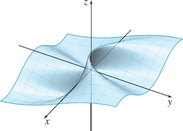
The graph of f(x,y) =\dfrac{x^{2}y}{x^{4}+y^{2}} is shown in Figure 24.
In Example 3, the limit failed to exist even though along all nonvertical lines the limit equals 0. We will see that this kind of behavior makes multivariable calculus different from single-variable calculus.
NOW WORK
How do we know a limit exists? The next example shows how to use the \varepsilon -\delta definition of a limit to prove that a limit exists.
824
EXAMPLE 4Showing That a Limit Exists
Use the \varepsilon -\delta definition of a limit to show that \lim\limits_{(x, y)\rightarrow (0, 0)}\dfrac{2xy^{2}}{x^{2}+y^{2}}=0.
Solution Given a number \varepsilon >0, we seek a number \delta >0, so that \begin{equation*} \hbox{whenever}\quad 0<\sqrt{(x-0) ^{2}+( y-0) ^{2}} <\delta \qquad \hbox{then}\quad \left\vert \dfrac{2xy^{2}}{x^{2}+y^{2}} -0\right\vert <\varepsilon \end{equation*}
That is, \begin{equation*} \hbox{whenever }\quad 0<\sqrt{x^{2}+y^{2}}<\delta \quad \hbox{then }\quad \left\vert \dfrac{2xy^{2}}{x^{2}+y^{2}}\right\vert <\varepsilon \end{equation*}
We need to find a connection between \dfrac{2xy^{2}}{x^{2}+y^{2}} and \sqrt{x^{2}+y^{2}}. We begin with the observation that since x^{2}\geq 0, \begin{equation*} y^{2}\leq x^{2}+y^{2}\hbox{ } \end{equation*}
So, for all points (x,y) not equal to (0,0), we have \dfrac{y^{2}}{x^{2}+y^{2}}\leq 1\qquad {\color{#0066A7}{\hbox{Divide both sides by \(x^2+y^2\).}}}
Now \begin{equation*} \left\vert \frac{2xy^{2}}{x^{2}+y^{2}}\right\vert =\frac{2\vert x\vert y^{2}}{x^{2}+y^{2}}=2\vert x\vert \cdot \dfrac{ y^{2}}{x^{2}+y^{2}}\leq 2\left\vert x\right\vert \cdot 1=2\sqrt{x^{2}}\leq 2 \sqrt{x^{2}+y^{2}} \end{equation*}
Given \varepsilon >0, we choose \delta \leq \dfrac{\varepsilon }{2}. Then whenever 0<\sqrt{x^{2}+y^{2}}<\delta , we have \begin{equation*} \left\vert \frac{2xy^{2}}{x^{2}+y^{2}}\right\vert \leq 2\sqrt{x^{2}+y^{2}} <2\delta \leq \varepsilon \end{equation*}
That is, \lim_{(x, y)\rightarrow (0, 0)}\left\vert \frac{2xy^{2}}{x^{2}+y^{2}} \right\vert =0 %%\tag{$\blacksquare \(}
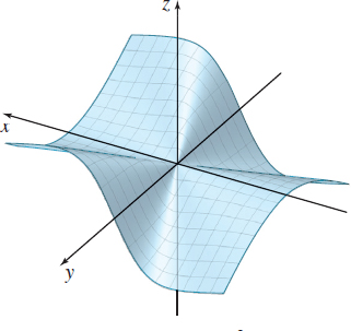
Figure 25 shows the graph of f(x,y) =\dfrac{2xy^{2}}{x^{2}+y^{2}}.
NOW WORK
As Example 4 illustrates, showing a limit exists using the \varepsilon -\delta definition can be challenging. For most of our work, we will not be required to show that limits exist in this way. We will instead find limits using various properties of functions, such as continuity.
4 Determine Whether a Function Is ContinuousPrinted Page 824
When investigating continuity for a function of one variable in Chapter 1, we began by defining what it means for a function f to be continuous at a number c, where f is defined on an open interval containing c. Then we extended the definition to include continuity on intervals: open, closed, or neither, and finally continuity on the domain of f.
NEED TO REVIEW?
Continuity for functions of one variable is discussed in Section 1.3, pp. 93-100.
For functions of two or three variables, we begin by defining continuity at a point in the plane or in space. But first, we need some preliminary definitions.
825
DEFINITION Interior Point; Boundary Point; Open Set; Closed Set
Let S be a set of points in the plane or in space.
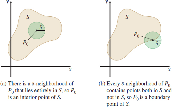
- A point P_{0} is called an interior point of S if there is a \delta -neighborhood of P_{0} that lies entirely in S.
- A point P_{0} is called a boundary point of S if every \delta -neighborhood of P_{0} contains points both in S and not in S. A boundary point of S may be in S or not in S.
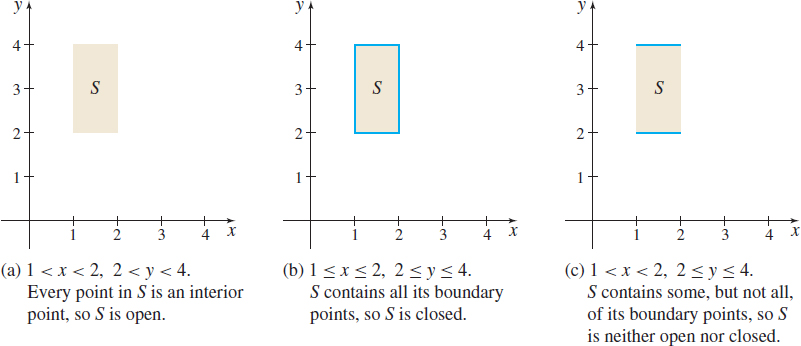
- A set S is called an open set if every point of S is an interior point.
- A set S is called a closed set if it contains all its boundary points.
- A set S that contains some, but not all, of its boundary points is neither open nor closed.
Figure 26(a) shows an interior point P_{0} in the set S. In Figure 26(b), the point P_{0} is a boundary point of S. Figure 27 shows an open set (a), a closed set (b), and a set that is neither open nor closed (c).
DEFINITION Continuity at a Point P_{0}
Let f be a function whose domain D is some subset of points in the plane, and let P_{0} be an interior point of D. Then f is continuous at P_{0} if the following two conditions are met:
- \lim\limits_{P\rightarrow P_{0}}f(P) exists
- \lim\limits_{P\rightarrow P_{0}}f(P)=f(P_{0})
826
If either one of the two conditions is not met, then we say that f is discontinuous at the point P_{0}.
If P_{0} is a boundary point of the domain D of f, then f is continuous at P_{0}, provided \lim\limits_{P\rightarrow P_{0}}f(P)=f(P_{0}) is taken to mean that given any \varepsilon >0, there is a \delta >0, so that whenever P is in the domain of f and d(P,P_{0})<\delta , then \left\vert f(P)-f(P_{0})\right\vert <\varepsilon .
DEFINITION Continuity on a Domain
A function f is continuous on its domain if it is continuous at every point in its domain. Such functions are referred to as continuous functions.
We use limit properties and information about continuous functions of one variable to obtain information about functions of two variables. For example, two important properties of continuous functions (of one or more variables) are:
- The sum, difference, product, or composition of two continuous functions is continuous.
- The quotient of two functions that are continuous at a point P_{0} is also continuous at P_{0}, provided the denominator is not 0 at P_{0}.
Let’s see how we use these properties. The function f(x,y) =ax^{n}y^{m}, where n and m are nonnegative integers and a is a constant, is continuous at every point (x,y) in the plane. This follows since \begin{eqnarray*} \lim\limits_{(x,y) \rightarrow (x_{0},y_{0}) }f(x,y) &=&\lim\limits_{(x,y) \rightarrow (x_{0},y_{0}) }( ax^{n}y^{m}) =\left[ \lim\limits_{(x,y) \rightarrow (x_{0},y_{0}) } ( ax^{n}) \right]\; \left[ \lim\limits_{(x,y) \rightarrow (x_{0},y_{0}) }y^{m}\right] \\[6pt] &=&a\left[ \lim\limits_{x\rightarrow x_{0}}\,x^{n}\right]\; \left[ \lim\limits_{y\rightarrow y_{0}}y^{m}\right] =ax_{0}^{n} y_{0}^{m} \end{eqnarray*}
Because a polynomial in two variables is a sum of functions of the form ax^{n}y^{m}, where n and m are nonnegative integers and a is a constant, it follows that polynomials in two variables are continuous at every point (x,y) in the plane. Further, rational functions, quotients of polynomials, are continuous on their domains, all points in the plane except those at which the denominator is 0.
EXAMPLE 5Determining Where a Function Is Continuous
Determine where the following functions are continuous:
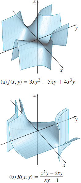
- (a) f(x,y) =3xy^{2}-5xy+4x^{3}y
- (b) R(x,y) =\dfrac{x^{2}y-2xy}{xy-1}
Solution (a) Since f is a polynomial function, it is continuous on its domain, every point (x,y) in the plane, as shown in Figure 28(a).
(b) R is a rational function and is continuous on its domain, all points (x,y) in the plane, except those for which xy=1. The graph of R will have no points on the cylinder xy=1, as shown in Figure 28(b).
NOW WORK
Another property of a continuous function is:
- The composite of a continuous function of one variable z=f( t) and a continuous function of two variables t=g(x,y) is continuous on its domain.
827
EXAMPLE 6Determining Where a Function Is Continuous
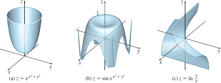
- (a) The function z=e^{t} is continuous for all t, and the function t=x^{2}+y^{2} is continuous on its domain (all points in the plane), so the composite z=e^{x^{2}+y^{2}} is continuous on its domain (all points in the plane), as shown in Figure 29(a).
- (b) The sine function z=\sin t is continuous for all t, and the function t=e^{x^{2}+y^{2}} is continuous for all points (x,y) in the plane, so the composite z=\sin e^{x^{2}+y^{2}} is continuous for all points (x,y) in the plane, as shown in Figure 29(b).
- (c) The function z=\ln t is continuous for all t>0, and the function t=\dfrac{y}{x} is continuous for all x\neq 0. The composite function z=\ln \dfrac{y}{x} is continuous for all (x,y) for which x>0, y>0 or x<0, y<0. The graph of z has no points for which x\geq 0, y\leq 0 or x\leq 0, y\geq 0, as shown in Figure 29(c).
NOW WORK
Finding limits of continuous functions can be done by substitution:
- If z=f(x,y) is continuous at the point (x_{0},y_{0}) , then \lim\limits_{(x,y) \rightarrow (x_{0},y_{0}) }f(x,y) =f(x_{0},y_{0})
EXAMPLE 7Finding Limits
- (a) \lim\limits_{(x,y) \rightarrow (0,0)}e^{x^{2}+y^{2}}\underset{\underset{\color{#0066A7}{\hbox{Example 6(a)}}}{\color{#0066A7}{\uparrow}}}{=}e^{0+0}=1
- (b) \lim\limits_{(x,y) \rightarrow ( \sqrt{\pi },0) }\sin e^{x^{2}+y^{2}}\underset{\underset{\color{#0066A7}{\hbox{Example 6(b)}}}{\color{#0066A7}{\uparrow}}}{=}\sin e^{\pi }
- (c) \lim\limits_{(x,y) \rightarrow (e,1) }\ln \dfrac{y}{x}\underset{\underset{\color{#0066A7}{\hbox{Example 6(c)}}}{\color{#0066A7}{\uparrow}}}{=}\ln \dfrac{1}{e}=\ln e^{-1}=-1