3.4 Differentials; Linear Approximations; Newton’s MethodPrinted Page 230
OBJECTIVES
When you finish this section, you should be able to:
1 Find the Differential of a Function and Interpret It GeometricallyPrinted Page 230
Recall that for a differentiable function y=f(x), the derivative is defined as dydx=f′(x)=lim
That is, for \Delta x sufficiently close to 0, we can make \dfrac{ \Delta y}{\Delta x} as close as we please to f^\prime (x). This can be expressed as \frac{\Delta y}{\Delta x}\approx f^\prime (x) \qquad \hbox{when}\qquad \Delta x\approx 0, \quad \Delta x≠ 0
231
or, since \Delta x≠ 0, as \bbox[5px, border:1px solid black, #F9F7ED]{ {\Delta y\approx f^\prime (x)\Delta x \qquad \hbox{when}\qquad \Delta x\approx 0, \quad \Delta x≠ 0}}\tag{1}
DEFINITION
Let y=f(x) be a differentiable function and let \Delta x denote a change in x.
The differential of x, denoted dx, is defined as dx=\Delta x≠ 0.
The differential of y, denoted dy, is defined as \bbox[5px, border:1px solid black, #F9F7ED]{ {dy=f^\prime (x) dx} }\tag{2}
From statement (1), if \Delta x \left( =dx\right) \approx 0, then \Delta y\approx dy=f^\prime (x) dx. That is, when the change \Delta x in x is close to 0, then the differential dy is an approximation to the change \Delta y in y.
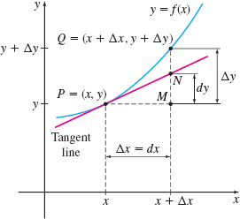
To see the geometric relationship between \Delta y and dy, we use Figure 8. There, P=(x, y) is a point on the graph of y=f(x) and Q=(x+\Delta x,y+\Delta y) is a nearby point also on the graph of f. The change \Delta y in y \Delta y=f( x+\Delta x) -f( x) is the distance from M to Q. The slope of the tangent line to f at P is f^\prime (x) =\dfrac{dy}{dx}. So numerically, the differential dy measures the distance from M to N. For \Delta x close to 0, dy=f^\prime (x) dx will be close to \Delta y.
EXAMPLE 1Finding and Interpreting Differentials Geometrically
For the function f(x) =xe^{x}:
- (a) Find the differential dy.
- (b) Compare dy to \Delta y when x=0 and \Delta x=0.5.
- (c) Compare dy to \Delta y when x=0 and \Delta x=0.1.
- (d) Compare dy to \Delta y when x=0 and \Delta x=0.01.
- (e) Discuss the results.
Solution (a) dy=f^\prime (x) dx= (xe^{x}+e^{x}) dx=(x+1) e^{x}dx.
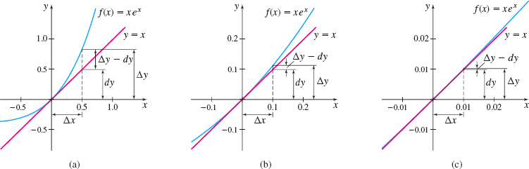
(b) See Figure 9(a). When x=0 and \Delta x=dx=0.5, then \ dy=(x+1) e^{x}dx=(0+1) e^{0}(0.5) =0.5


232
The tangent line rises by 0.5 as x changes from 0 to 0.5. The corresponding change in the height of the graph f is \begin{eqnarray*} \Delta y=f( x+\Delta x) -f( x) &=&f(0.5) -f( 0) =0.5e^{0.5}-0\approx 0.824\\ \vert \Delta y-dy\vert &\approx& \vert 0.824-0.5\vert =0.324 \end{eqnarray*}
The graph of the tangent line is approximately 0.324 below the graph of f at x\,{=}\,0.5.
(c) See Figure 9(b). When x=0 and \Delta x=dx=0.1, then dy=(0+1) e^{0}(0.1) =0.1
The tangent line rises by 0.1 as x changes from 0 to 0.1. The corresponding change in the height of the graph f is \begin{eqnarray*} \Delta y=f( x+\Delta x) -f( x) &=&f(0.1) -f( 0) =0.1e^{0.1}-0\approx 0.111\\ \vert \Delta y-dy\vert &\approx& \left\vert 0.111-0.1\right\vert =0.011 \end{eqnarray*}
The graph of the tangent line is approximately 0.011 below the graph of f at x=0.1.
(d) See Figure 9(c). When x=0 and \Delta x=dx=0.01, then dy=(0+1) e^{0}( 0.01) =0.01
The tangent line rises by 0.01 as x changes from 0 to 0.01. The corresponding change in the height of the graph of f is \begin{eqnarray*} \Delta y=f( x+\Delta x) -f( x) &=&f( 0.01) -f( 0) =0.01e^{0.01}-0\approx 0.0101\\ \vert \Delta y-dy\vert &\approx& \vert 0.0101-0.01\vert =0.0001 \end{eqnarray*}
The graph of the tangent line is approximately 0.0001 below the graph of f at x=0.01.
(e) The closer \Delta x is to 0, the closer dy is to \Delta y. So, we conclude that the closer \Delta x is to 0, the less the tangent line departs from the graph of the function. That is, we can use the tangent line to f at a point P as a linear approximation to f near P.
NOW WORK
Example 1 shows that when dx is close to 0, the tangent line can be used as a linear approximation to the graph. We discuss next how to find this linear approximation.
2 Find the Linear Approximation to a FunctionPrinted Page 232
Suppose y=f( x) is a differentiable function and suppose ( x_{0},y_{0}) is a point on the graph of f. Then \Delta y=f( x) -f( x_{0})\qquad \hbox{and}\qquad dy=f^\prime (x_{0})dx=f^\prime (x_{0})\Delta x=f^\prime (x_{0})(x-x_{0})
If dx=\Delta x is close to 0, then \begin{eqnarray*} \Delta y &\approx & dy \\ f(x)-f({x_{0}}) &\approx & f^\prime ({x_{0}})({x-x_{0}}) \\ f(x) &\approx & f({x_{0}})+f^\prime ({x_{0}})({x-x_{0}}) \end{eqnarray*}
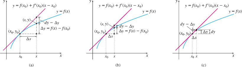
See Figure 10. Each figure shows the graph of y=f( x) and the graph of the tangent line at (x_{0},y_{0}). The first two figures show the difference between \Delta y and dy. The third figure illustrates that when \Delta x is close to 0, \Delta y\approx dy.
THEOREM Linear Approximation
The linear approximation {L( x)} to a differentiable function f at x=x_{0} is given by \bbox[5px, border:1px solid black, #F9F7ED]{L( x) =f( x_{0}) +f^\prime ( x_{0}) ( x-x_{0})} \tag{3}
The closer x is to x_{0}, the better the approximation. The graph of the linear approximation y=L( x) is the tangent line to the graph of f at x_{0}, and L is often called the linearization of {f} at x_{0}. Although L provides a good approximation of f in an interval centered at x_{0}, the next example shows that as the interval widens, the accuracy of the approximation of L may decrease. In Section 3.5, we use higher-degree polynomials to extend the interval for which the approximation is efficient.
233

EXAMPLE 2Finding the Linear Approximation to a Function
- (a) Find the linear approximation L( x) to f(x)=\sin x near x=0.
- (b) Use L( x) to approximate \sin \left( -0.3\right) , \sin 0.1 , \sin 0.4, \sin 0.5 , and \sin \dfrac{\pi }{4}.
- (c) Graph f and L.
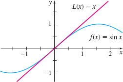
Solution (a) Since f^\prime ( x) =\cos x, then f(0)=\sin 0=0 and f^\prime (0) = \cos 0 = 1. Using Equation (3), the linear approximation L( x) to f at 0 is L( x) =f(0) + f^\prime (0)(x -0)=x
So, for x close to 0, the function f( x) =\sin x can be approximated by the line L( x) =x.
(b) The approximate values of \sin x using L( x) =x, the true values of \sin x, and the absolute error in using the approximation are given in Table 3. From Table 3, we see that the further x is from 0, the worse the line L( x) =x approximates f( x) =\sin x.
| {L(x) =x} | {f(x) =\sin x} | Error: {\vert x-\sin x\vert} |
| 0.1 | 0.0998 | 0.0002 |
| -0.3 | -0.2955 | 0.0045 |
| 0.4 | 0.3894 | 0.0106 |
| 0.5 | 0.4794 | 0.0206 |
| \dfrac{\pi }{4}\approx 0.7854 | 0.7071 | 0.0783 |
(c) See Figure 11 for the graphs of f( x) =\sin x and L( x) =x.
NOW WORK
The next two examples show applications of differentials. In these examples, we use the differential to approximate the change.
3 Use Differentials in ApplicationsPrinted Page 233
EXAMPLE 3Measuring Metal Loss in a Mechanical Process
A spherical bearing has a radius of 3{\,{\rm{cm}}} when it is new. Use differentials to approximate the volume of the metal lost after the bearing wears down to a radius of 2.971{\,{\rm{cm}}}. Compare the approximation to the actual volume lost.

Solution The volume V of a sphere of radius R is V=\dfrac{4}{3}\pi R^{3}. As a machine operates, friction wears away part of the bearing. The exact volume of metal lost equals the change \Delta V in the volume V of the sphere, when the change in the radius of the bearing is \Delta R=2.971-3={-}0.029{\,{\rm{cm}}}. Since the change \Delta R is small, we use the differential dV to approximate the change \Delta V. Then \begin{eqnarray*} && \Delta V \approx dV \underset{\underset{\color{#0066A7}{\hbox{\(dV=V^{\,\prime} dR\)}}}{\color{#0066A7}{\uparrow }}}{=} 4\pi R^{2}dR \underset{\underset{\color{#0066A7}{\hbox{\(dR=\Delta R\)}}}{\color{#0066A7}{\uparrow}}}{=} (4\pi )(3^{2})({-} 0.029) \approx {-}3.280 \end{eqnarray*}
The approximate loss in volume of the bearing is 3.28{\,{\rm{cm}}}^{3}.
234
The actual loss in volume \Delta V is \Delta V=V(R+\Delta R)-V(R)=\dfrac{4}{3}\pi \cdot 2.971^{3}-\dfrac{4}{3}\pi \cdot 3^{3}=\dfrac{4}{3}\pi ( -0.7755) =-3.248{\,{\rm{cm}}}^{3}
The approximate change in volume is correct to one decimal place.
NOW WORK
The use of dy to approximate \Delta y when \Delta x= dx is small is also helpful in approximating error. If Q is the quantity to be measured and if \Delta Q is the change in Q, then the \bbox[5px, border:1px solid black, #F9F7ED]{ {\begin{array}{@{}rcl@} \hbox{Relative error at \(x_0\) in \(Q\)}&=&\dfrac{ \vert \Delta Q\vert } {Q( x_{0}) } \\ \hbox{Percentage error at \(x_0\) in \(Q\)} &=&\dfrac{\vert \Delta Q\vert }{Q( x_{0}) }\cdot 100\% \end{array}}}
For example, if Q=50 units and the change \Delta Q in Q is measured to be 5 units, then \hbox{Relative error at }50 \hbox{ in}\ Q=\frac{5}{50}=0.10\qquad\! \hbox{Percentage error at }50\hbox{ in }Q=10\%
When \Delta x is small, dQ\approx \Delta Q. The relative error and percentage error at x_{0} in Q can be approximated by \dfrac{\vert dQ\vert }{Q( x_{0}) } and \dfrac{\vert dQ\vert }{Q( x_{0}) }\cdot 100\%, respectively.
EXAMPLE 4Measuring Error in a Manufacturing Process
A company manufactures spherical ball bearings of radius 3{\,{\rm{cm}}}. The customer accepts a tolerance of 1% in the radius. Use differentials to approximate the relative error for the surface area of the acceptable ball bearings.
Solution The tolerance of 1% in the radius R means that the relative error in the radius R must be within 0.01. That is, \dfrac{\vert \Delta R\vert }{R}≤ 0.01. The surface area S of a sphere of radius R is given by the formula S=4\pi R^{2}. We seek the relative error in S, \dfrac{\vert \Delta S\vert }{S}, which can be approximated by \dfrac{\vert dS\vert}{S}. \begin{eqnarray*} && \frac{\vert \Delta S\vert }{S}\approx \frac{\vert dS\vert }{S} \underset{\underset{\color{#0066A7}{\hbox{\(dS=S^{\,\prime} dR\)}}}{\color{#0066A7}{\uparrow}}}{=} \frac{( 8\pi R) \vert dR \vert }{4\pi R^{2}}=\frac{2\vert dR\vert }{R}= 2\cdot \frac{\vert \Delta R\vert }{R} \underset{\underset{\color{#0066A7}{\hbox{\(\tfrac{\vert \Delta R\vert }{R}≤ 0.01\)}}}{\color{#0066A7}{ \uparrow}}}{\le} 2(0.01)= 0.02 \end{eqnarray*}
The relative error in the surface area will be less than or equal to 0.02.
In Example 4, the tolerance of 1% in the radius of the ball bearing means the radius of the sphere must be somewhere between 3-0.01( 3) =2.97{\,{\rm{cm}}} and 3+0.01( 3) =3.03{\,{\rm{cm}}}. The corresponding 2% error in the surface area means the surface area lies within \pm0.02 of S=4\pi R^{2}=36\pi {\,{\rm{cm}}}^{2}. That is, the surface area is between 35.28\pi \approx 110.84{\,{\rm{cm}}}^{2} and 36.72\pi \approx 115.36{\,{\rm{cm}}}^{2}. Notice that a rather small error in the radius results in a more significant variation in the surface area!
NOW WORK
4 Use Newton’s Method to Approximate a Real Zero of a FunctionPrinted Page 234
Newton’s Method is used to approximate a real zero of a function. Suppose a function y=f(x) is defined on a closed interval [a, b] , and its derivative f^\prime is continuous on the interval ( a, b) . Also suppose that, from the Intermediate Value Theorem or from a graph or by trial calculations, we know that the function f has a real zero in some open subinterval of (a, b) containing the number c_{1}.
235
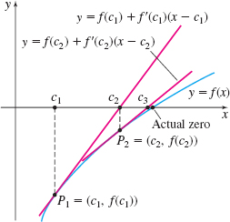
Draw the tangent line to the graph of f at the point P_{1}=(c_{1}, f(c_{1})) and label as c_{2} the x-intercept of the tangent line. See Figure 12. If c_{1} is a first approximation to the required zero of f, then c_{2} will be a better, or second approximation to the zero. Repeated use of this procedure often* generates increasingly accurate approximations to the zero we seek.
Suppose c_{1} has been chosen. We seek a formula for finding the approximation c_{2}. The coordinates of P_{1} are ( c_{1}, f(c_{1}) ) , and the slope of the tangent line to the graph of f at point P_{1} is f^\prime (c_{1}). So, the equation of the tangent line to graph of f at P_{1} is y-f(c_{1})=f^\prime (c_{1})(x-c_{1})
To find the x-intercept c_{2}, we let y=0. Then c_{2} satisfies the equation \begin{eqnarray*} \begin{array}{rl@{\qquad}l} -f( c_{1}) &= f^\prime ( c_{1}) ( c_{2}-c_{1})\\ c_{2}&= c_{1}-\dfrac{f(c_{1})}{f^\prime (c_{1})}\qquad \hbox{if } f^\prime (c_{1}) ≠ 0 & {{\color{#0066A7}{\hbox{Solve for }c_2.}}} \end{array} \end{eqnarray*}
Notice that we are using the linear approximation to f at the point (c_{1},f( c_{1}) ) to approximate the zero.
Now repeat the process by drawing the tangent line to the graph of f at the point P_{2}=(c_{2},f( c_{2}) ) and label as c_{3} the x-intercept of the tangent line. By continuing this process, we have Newton’s method.
*See When Newton’s Method Fails, after Example 6.
Newton’s Method
Suppose a function f is defined on a closed interval [a, b] and its first derivative f^\prime is continuous and not equal to 0 on the open interval ( a, b) . If x=c_{1} is a sufficiently close first approximation to a real zero of the function f in ( a, b) , then the formula \bbox[5px, border:1px solid black, #F9F7ED]{ c_{2}=c_{1}-\dfrac{f(c_{1})}{f^\prime (c_{1})}} gives a second approximation to the zero. The nth approximation to the zero is given by \bbox[5px, border:1px solid black, #F9F7ED]{ c_{n}=c_{n-1}-\dfrac{f( c_{n-1}) }{f^\prime (c_{n-1})}}
ORIGINS
When Isaac Newton first introduced his method for finding real zeros in 1669, it was very different from what we did here. Newton’s original method (also known as the Newton–Raphson Method) applied only to polynomials, and it did not use calculus! In 1690 Joseph Raphson simplified the method and made it recursive, again without calculus. It was not until 1740 that Thomas Simpson used calculus, giving the method the form we use here.
The formula in Newton’s Method is a recursive formula, because the approximation is written in terms of the previous result. Since recursive processes are particularly useful in computer programs, variations of Newton’s Method are used by many computer algebra systems and graphing utilities to find the zeros of a function.
EXAMPLE 5Using Newton’s Method to Approximate a Real Zero of a Function
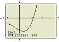
Use Newton’s Method to find a fourth approximation to the positive real zero of the function f( x) =x^{3}+x^{2}-x-2.
Solution Since f(1) =-1 and f(2) =8, we know from the Intermediate Value Theorem that f has a zero in the interval (1, 2) . Also, since f is a polynomial function, both f and f^\prime are differentiable functions. Now f(x) =x^{3}+x^{2}-x-2 \qquad \hbox{and}\qquad f^\prime ( x) =3x^{2}+2x-1
236
We choose c_{1}=1.5 as the first approximation and use Newton’s Method. The second approximation to the zero is c_{2}=c_{1}-\dfrac{f( c_{1}) }{f^\prime ( c_{1}) }=1.5-\dfrac{f(1.5) }{f^\prime (1.5) }=1.5-\dfrac{2.125}{ 8.75}\approx 1.2571429
Use Newton’s Method again, with c_{2}=1.2571429. Then f(1.2571429) \approx 0.3100644 and f^\prime (1.2571429)\approx 6.2555106. The third approximation to the zero is c_{3}=c_{2}-\dfrac{f( c_{2}) }{f^\prime ( c_{2}) }=1.2571429-\dfrac{0.3100641}{6.2555102}\approx 1.2075763
The fourth approximation to the zero is c_{4}=c_{3}-\dfrac{f( c_{3}) }{f^\prime ( c_{3}) } =1.2075763-\dfrac{0.0116012}{5.7898745}\approx 1.2055726
Using graphing technology, the zero of f( x) =x^{3}+x^{2}-x-2 is given as x=1.2055694. See Figure 13.
NOW WORK
The table feature of a graphing utility can be used to take advantage of the recursive nature of Newton’s Method and speed up the computation.
EXAMPLE 6Using Technology with Newton’s Method
![]() The graph of the function f( x) =\sin x+x^{2}-1 is shown in Figure 14.
The graph of the function f( x) =\sin x+x^{2}-1 is shown in Figure 14.
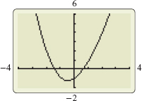
- (a) Use the Intermediate Value Theorem to confirm that f has a zero in the interval (0,1) .
- (b) Use graphing technology with Newton’s Method and a first approximation of c_{1}= 0.5 to find a fourth approximation to the zero.
Solution (a) The function f( x) =\sin x+x^{2}-1 is continuous on its domain, all real numbers, so it is continuous on the closed interval [0,1] . Since f( 0) =-1 and f(1) =\sin 1\approx 0.841 have opposite signs, the Intermediate Value Theorem guarantees that f has a zero in the interval (0,1) .
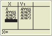
(b) We begin by finding f^\prime ( x) =\cos x+2x. To use Newton’s Method with a graphing utility, we enter x-\dfrac{\sin x+x^{2}-1}{\cos x+2x} \qquad {\color{#0066A7}{x-\dfrac{{ f}({x}) }{{ f^\prime }({x})}}}
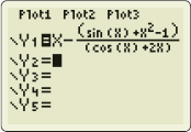
into the Y= \hbox{editor}, as shown in Figure 15. We create a table by entering the initial value 0.5 in the X column. The graphing utility computes 0.5-\dfrac{\sin 0.5+0.5^{2}-1}{\cos 0.5+2(0.5) }=0.64410789
and displays 0.64411 in column Y_{1} next to 0.5. The value Y_{1} is the second approximation c_{2} that we use in the next iteration. That is, we enter 0.64410789 in the X column of the next row, and the new entry in column Y_{1} is the third approximation c_{3}. We repeat the process until we obtain the desired approximation. The fourth approximation to the zero of f is 0.63673, as shown in Figure 16.
NOW WORK
When Newton’s Method Fails
You may wonder, does Newton’s Method always work? The answer is no, as we mentioned earlier. The list below, while not exhaustive, gives some conditions under which Newton’s Method fails.
237
- Newton’s Method fails if the conditions of the theorem are not met
- (a) f^\prime (c_{n}) =0: Algebraically, division by 0 is not defined. Geometrically, the tangent line is parallel to the x-axis and so has no x-intercept.
- (b) f^\prime ( c) is undefined: The process cannot be used.
- Newton’s Method fails if the initial estimate c_{1} may not be “good enough:”
- (a) Choosing an initial estimate too far from the required zero could result in approximating a different zero of the function.
- (b) The convergence could approach the zero so slowly that hundreds of iterations are necessary.
- Newton’s Method fails if the terms oscillate between two values and so never get closer to the zero.
Problems 72–75 illustrate some of these possibilities.