10.3 Vectors in the Plane and in SpacePrinted Page 703
OBJECTIVES
When you finish this section, you should be able to:
We have been treating vectors geometrically, but to use vectors in a meaningful way, we need to look at vectors algebraically as well. To do this, we use a rectangular coordinate system: with two dimensions for vectors in the plane and with three dimensions for vectors in space.
1 Represent a Vector AlgebraicallyPrinted Page 703
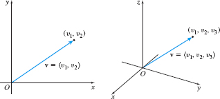
If v is a vector in a plane, and if its initial point is at the origin and its terminal point is at the point (v1,v2), then we may represent v by the ordered pair. \bbox[5px, border:1px solid black, #F9F7ED]{ \mathbf{v~}=\left\langle v_{1},v_{2}\right\rangle }
The numbers v_{1} and v_{2} are called the components of \mathbf{v}.
Similarly, if \mathbf{v} is a vector in space with its initial point at the origin and its terminal point at the point ( v_{1},\,v_{2},\,v_{3}) , then \mathbf{v} is represented by the ordered triple. \bbox[5px, border:1px solid black, #F9F7ED]{ \mathbf{v~}=\left\langle v_{1},v_{2},v_{3}\right\rangle }
The numbers v_{1}, v_{2}, and v_{3} are called the components of \mathbf{v}.
The vectors defined here, as well as any other vector whose initial point is at the origin, are called position vectors. See Figure 25 on page 704.
704
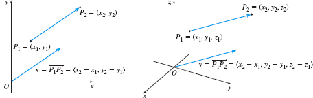
Any vector whose initial point is not at the origin is equal to a unique position vector. If \mathbf{v} is a vector in the plane with initial point P_{1}=( x_{1},\,y_{1}) and terminal point P_{2}=( x_{2},\,y_{2}) , then \mathbf{v} equals the position vector \bbox[5px, border:1px solid black, #F9F7ED]{ \mathbf{v=\,}\left\langle x_{2}-x_{1},\,y_{2}-y_{1}\right\rangle }
Similarly, if \mathbf{v} is a vector in space with initial point P_{1}= ( x_{1},\,y_{1},\,z_{1}) and terminal point P_{2}=( x_{2},\,y_{2},\,\,z_{2}) , then \mathbf{v} equals the position vector \bbox[5px, border:1px solid black, #F9F7ED]{ \mathbf{v=\,}\left\langle x_{2}-x_{1},\,y_{2}-y_{1},\,z_{2}-z_{1}\right\rangle }
As Figure 26 illustrates, this feature allows us to move vectors around in applications.
IN WORDS
Every vector can be represented by a unique vector whose initial point is at the origin.
If both the initial point and the terminal point of vector \mathbf{v} are at the origin, then \mathbf{v} is the zero vector. As a result, \bbox[5px, border:1px solid black, #F9F7ED]{ \mathbf{0\,=~}\left\langle 0,0\right\rangle \hbox{in the plane}\qquad \text{and}\qquad \mathbf{0=\,}\left\langle 0,0,0\right\rangle \hbox{in space} }
EXAMPLE 1Finding a Position Vector
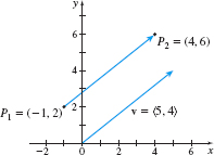
Find the unique position vector \mathbf{v} of a vector whose initial point is P_{1} and whose terminal point is P_{2}.
- (a) P_{1}=(-1,2),\quad P_{2}=(4,6)
- (b) P_{1}=(3,4,2),\quad P_{2}=(7,-8,5)
Solution To find \mathbf{v}, subtract corresponding components.
- (a) Then \mathbf{v}=\langle 4-(-1), 6-2\rangle =\langle 5,4\rangle , as shown in Figure 27.
- (b) Here, \mathbf{v}=\langle 7-3,-8-4,5-2\rangle =\langle 4,-12,3\rangle
NOW WORK
705
Two position vectors \mathbf{v} and \mathbf{w} are equal if and only if the terminal point of \mathbf{v} is the same as the terminal point of \mathbf{w}. \bbox[5px, border:1px solid black, #F9F7ED]{ \mathbf{v}=\langle v_{1},v_{2}\rangle\, \hbox{and}\, \mathbf{w}=\langle w_{1},w_{2}\rangle\,\hbox{are equal if and only if}\, v_{1}=w_{1}\, \hbox{and}\, v_{2}=w_{2}. }
Unless otherwise specified, we will represent a vector by the unique position vector equal to it.
2 Add, Subtract, and Find Scalar Multiples of VectorsPrinted Page 705
In Section 10.2, we described the operations of addition, subtraction, and scalar multiplication geometrically. Here, we present them algebraically.
Vectors are added or subtracted and scalar multiples are formed using the components of the vectors.
DEFINITION Operations with Vectors
If \mathbf{v}=\langle v_{1},v_{2}\rangle and \mathbf{w}=\langle w_{1},w_{2}\rangle are two vectors in the plane and if a is a scalar, then
- \mathbf{v}+\mathbf{w}=\langle v_{1}+w_{1}, v_{2}+w_{2}\rangle
- \mathbf{v}-\mathbf{w}=\langle v_{1}-w_{1}, v_{2}-w_{2}\rangle
- a\,\mathbf{v}=\langle av_{1}, av_{2}\rangle
If \mathbf{v}=\langle v_{1}, v_{2}, v_{3}\rangle and \mathbf{w}=\langle w_{1}, w_{2}, w_{3}\rangle are two vectors in space and if a is a scalar, then
- \mathbf{v}+\mathbf{w}=\langle v_{1}+w_{1},v_{2}+w_{2},v_{3}+w_{3}\rangle
- \mathbf{v}-\mathbf{w}=\langle v_{1}-w_{1},v_{2}-w_{2},v_{3}-w_{3}\rangle
- a\,\mathbf{v}=\langle av_{1},av_{2},av_{3}\rangle
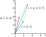
For example, if \mathbf{v}=\langle 2,3\rangle and \mathbf{w}=\langle 1,4\rangle , then \mathbf{v}+\mathbf{w}=\langle 2+1,3+4\rangle =\langle 3,7\rangle . See Figure 28.
Notice that the algebraic sum \mathbf{v}+\mathbf{w} is the same as the resultant vector obtained geometrically. In other words, the algebraic representation of vectors agrees with the geometric representation discussed in Section 10.2.
EXAMPLE 2Adding and Subtracting Vectors Algebraically
If \mathbf{v}=\langle 2,3,-1\rangle and \mathbf{w}=\langle -1,-2, 4\rangle , find:
- (a) \mathbf{v}+\mathbf{w}
- (b) \mathbf{w-v}
- (c) \dfrac{1}{2}\mathbf{w}
- (d) 2\mathbf{v}+3\mathbf{w}
Solution
(a) \mathbf{v} + \mathbf{w} = \langle 2,3,-1\rangle +\langle -1,-2,4\rangle =\left\langle 2+(-1), 3+(-2), -1+4\right\rangle =\langle 1,1,3\rangle
(b) \mathbf{w-v=} \langle -1,-2,4\rangle - \langle 2,3,-1\rangle =\left\langle -1-2, -2-3, 4-( -1) \right\rangle =\left\langle -3,-5,5\right\rangle
(c) \dfrac{1}{2}\mathbf{w}=\dfrac{1}{2}\,\langle -1,-2,4\rangle = \left\langle \dfrac{1}{2}( -1), \dfrac{1}{2} ( -2), \dfrac{1}{2}(4) \right\rangle = \left\langle -\dfrac{1}{2},-1,2\right\rangle
(d) 2\mathbf{v} + 3\mathbf{w} = 2\,\langle 2,3,-1\rangle+3\,\langle -1,-2,4\rangle =\langle 4,6,-2\rangle +\langle -3,-6,12\rangle =\langle 1,0,10\rangle
NOW WORK
706
The properties listed below for vectors are similar to the properties of real numbers.
THEOREM Properties of Vector Addition and Scalar Multiplication
If \mathbf{u}, \mathbf{v}, and \mathbf{w} are vectors and if a and b are scalars, then the following properties hold:
- Commutative property of vector addition: \bbox[5px, border:1px solid black, #F9F7ED]{ \mathbf{u}+\mathbf{v}=\mathbf{v}+\mathbf{u}}
- Associative property of vector addition: \bbox[5px, border:1px solid black, #F9F7ED]{ \mathbf{u}+(\mathbf{v}+\mathbf{w})=(\mathbf{u}+\mathbf{v})+\mathbf{w} }
- Additive identity \mathbf{0}: \bbox[5px, border:1px solid black, #F9F7ED]{ \mathbf{v}+\mathbf{0}=\mathbf{0}+\mathbf{v}=\mathbf{v} }
- Additive inverse property: \bbox[5px, border:1px solid black, #F9F7ED]{ \mathbf{v}+(-\mathbf{v})=\mathbf{0} }
- Distributive property of scalar multiplication over vector addition: \bbox[5px, border:1px solid black, #F9F7ED]{ a( \mathbf{u}+\mathbf{v}) =a\,\mathbf{u}+a\,\mathbf{v} }
- Distributive property of scalar multiplication over scalar addition: \bbox[5px, border:1px solid black, #F9F7ED]{ ( a+b) \mathbf{v}=a\,\mathbf{v}+b\,\mathbf{v} }
- Linearity property of scalar multiplication: \bbox[5px, border:1px solid black, #F9F7ED]{ a( b\,\mathbf{v}) =( ab) \mathbf{v} }
- Scalar multiplication identity: \bbox[5px, border:1px solid black, #F9F7ED]{ 1\mathbf{v}=\mathbf{v}}
We proved some of these properties geometrically. For example, in Figure 18, we gave a geometric proof of the commutative property of addition. Here, we algebraically prove the commutative property for vectors in the plane and the scalar multiplication identity property for vectors in space. The remaining proofs are left as exercises. See Problems 106 and 107.
Proof
Commutative property of vector addition (in the plane) : If \mathbf{u}=\langle u_{1},u_{2}\rangle and if \mathbf{v} =\langle v_{1},v_{2}\rangle , then \begin{eqnarray*} \mathbf{u}+\mathbf{v}&=&\langle u_{1},u_{2}\rangle +\langle v_{1},v_{2}\rangle =\langle u_{1}+v_{1},u_{2}+v_{2}\rangle =\langle v_{1}+u_{1},v_{2}+u_{2}\rangle\\[4pt] &=&\langle v_{1},v_{2}\rangle +\langle u_{1},u_{2}\rangle =\mathbf{v}+\mathbf{u} \end{eqnarray*}
Scalar multiplication identity (in space): If \mathbf{v}=\langle v_{1}, v_{2}, v_{3}\rangle , then \begin{equation*} 1\mathbf{v}=\langle 1v_{1}, 1v_{2}, 1v_{3}\rangle =\langle v_{1}, v_{2}, v_{3}\rangle =\mathbf{v} \end{equation*}
DEFINITION Parallel Vectors
Let \mathbf{v} and \mathbf{w} be two distinct nonzero vectors. If there is a nonzero scalar a for which \mathbf{v}=a\,\mathbf{w}, then \mathbf{v} and \mathbf{w} are called parallel vectors.
707
EXAMPLE 3Showing Two Vectors Are Parallel
- (a) The vectors \begin{equation*} \mathbf{v}=\langle 2,3,-1\rangle\qquad\hbox{and}\qquad\mathbf{w}=\langle 4,6,-2\rangle \end{equation*} are parallel, since \mathbf{v}=\dfrac{1}{2}\mathbf{w}. In this case, \mathbf{v} and \mathbf{w} have the same direction.
- (b) The vectors \begin{equation*} \mathbf{v}=\left\langle 1,2,3\right\rangle\qquad \hbox{and}\qquad\mathbf{w}=\langle -3,-6,-9\rangle \end{equation*} are parallel, since \mathbf{w}=-3\,\mathbf{v}. In this case, \mathbf{v} and \mathbf{w} have opposite directions.
NOW WORK
3 Find the Magnitude of a VectorPrinted Page 707
The representation of \mathbf{v} as the vector \langle v_{1},v_{2}\rangle gives the direction of \mathbf{v}. The definition below gives the magnitude of \mathbf{v}.
DEFINITION
The magnitude or length of a vector \mathbf{v}, denoted by the symbol \Vert \mathbf{v}\Vert , is the distance from the initial point to the terminal point of \mathbf{v}. \Vert \mathbf{v}\Vert is also called the norm of the vector \mathbf{v}.
THEOREM Magnitude of a Vector
If \mathbf{v}=\langle v_{1},v_{2}\rangle is a vector in the plane, the magnitude of \mathbf{v} is \bbox[5px, border:1px solid black, #F9F7ED]{ \Vert \mathbf{v}\Vert \,=\sqrt{v_{1}^{2}+v_{2}^{2}}}
If \mathbf{v}=\langle v_{1},v_{2},v_{3}\rangle is a vector in space, the magnitude of \mathbf{v} is \bbox[5px, border:1px solid black, #F9F7ED]{ \Vert \mathbf{v}\Vert \,=\sqrt{v_{1}^{2}+v_{2}^{2}+v_{3}^{2}} }
The proof follows from the Distance Formula.
EXAMPLE 4Finding the Magnitude of a Vector
Find the magnitude of \mathbf{v} if:
- (a) \mathbf{v} = \langle 3,-4\rangle
- (b) \mathbf{v}=\langle 2,3,-1\rangle
Solution (a) \Vert \mathbf{v}\Vert = \sqrt{v_{1}^{2}+v_{2}^{2}} = \sqrt{3^{2}+(-4)^{2}} = \sqrt{9+16} = 5
(b) \Vert \mathbf{v}\Vert = \sqrt{v_{1}^{2} + v_{2}^{2} + v_{3}^{2}} = \sqrt{2^{2} + 3^{2} + (-1)^{2}} = \sqrt{4 + 9 + 1} = \sqrt{14}
NOW WORK
THEOREM Magnitude of the Scalar Multiple of a Vector
If a is scalar and \mathbf{v} is a vector, then \bbox[5px, border:1px solid black, #F9F7ED]{ \Vert a \mathbf{v}\Vert = |a| \Vert \mathbf{v}\Vert}
We prove the theorem for a vector \mathbf{v} in the plane. The proof for a vector \mathbf{v} in space is left as an exercise (Problem 108).
708
Proof
Suppose \mathbf{v} = \langle v_{1}, v_{2}\rangle. Then the scalar multiple of a and \mathbf{v} is a\mathbf{v} = \langle av_{1}, av_{2}\rangle and \begin{eqnarray*} \Vert a\mathbf{v}\Vert &=& \sqrt{(av_{1})^{2} + (av_{2})^{2}} = \sqrt{a^{2}v_{1}^{2} + a^{2}v_{2}^{2}} = \sqrt{a^{2}\big(v_{1}^{2} + v_{2}^{2}\big)}\\[4pt] &=&\sqrt{a^{2}}\sqrt{v_{1}^{2} + v_{2}^{2}} = |a| \Vert v\Vert \end{eqnarray*}
4 Find a Unit VectorPrinted Page 708
DEFINITION
A vector with magnitude 1 is called a unit vector.
In many applications, it is necessary to find the unit vector with the same direction as a given vector \mathbf{v}.
THEOREM Unit Vector in the Direction of \mathbf{v}
For any nonzero vector \mathbf{v}, the vector \bbox[5px, border:1px solid black, #F9F7ED]{ \mathbf{u}=\dfrac{\mathbf{v}}{\Vert \mathbf{v\Vert }}}
is the unit vector that has the same direction as \mathbf{v}.
Proof
Since \dfrac{1}{\Vert \mathbf{v}\Vert} is a positive scalar, the vector \mathbf{u} = \dfrac{1}{\Vert \mathbf{v}\Vert} \mathbf{v} has the same direction as \mathbf{v}. Next we show that the magnitude of \mathbf{u} is 1.
\begin{eqnarray*} \Vert \mathbf{u}\Vert =\left\Vert \dfrac{\mathbf{v}}{\Vert \mathbf{v\Vert }} \right\Vert =\left\Vert \dfrac{1}{\Vert \mathbf{v\Vert }}\mathbf{v} \right\Vert =\dfrac{1}{\Vert \mathbf{v\Vert }}\left\Vert \mathbf{v} \right\Vert =1 \end{eqnarray*}
Since \Vert \mathbf{u}\Vert =1, \mathbf{u} is a unit vector in the direction of \mathbf{v}.
Multiplying a nonzero vector \mathbf{v} by \dfrac{1}{\Vert \mathbf{v}\Vert } to obtain a unit vector that has the same direction as \mathbf{v} is called normalizing \mathbf{v}.

EXAMPLE 5Normalizing a Vector
Normalize each vector. That is, find a unit vector \mathbf{u} that has the same direction as:
- (a) \mathbf{v} = \langle 3,-4\rangle
- (b) \mathbf{v} = \langle -1,2,-2\rangle
Solution (a) Since \mathbf{v} = \langle 3,-4\rangle, then \Vert \mathbf{v}\Vert = \sqrt{9 + 16} = 5. The unit vector \mathbf{u} in the same direction as \mathbf{v} is \begin{eqnarray*} \mathbf{u} = \dfrac{\mathbf{v}}{\Vert \mathbf{v\Vert }} = \dfrac{\mathbf{v}}{5} = \left\langle \dfrac{3}{5}, -\dfrac{4}{5}\right\rangle \end{eqnarray*}
(b) Since \mathbf{v} = \langle -1,2,-2\rangle, then \Vert \mathbf{v}\Vert = \sqrt{1 + 4 + 4} = 3. The unit vector \mathbf{u} in the same direction as \mathbf{v} is \begin{eqnarray*} \mathbf{u} = \dfrac{\mathbf{v}}{\Vert \mathbf{v\Vert }} = \dfrac{\mathbf{v}}{3} = \left\langle -\dfrac{1}{3}, \dfrac{2}{3}, -\dfrac{2}{3}\right\rangle \end{eqnarray*}
NOW WORK
Unit vectors directed along the positive coordinate axes are called standard basis vectors. In the plane, the standard basis vectors are \bbox[5px, border:1px solid black, #F9F7ED]{ \mathbf{i} = \langle 1,0\rangle\qquad \mathbf{j} = \langle 0,1\rangle}
709
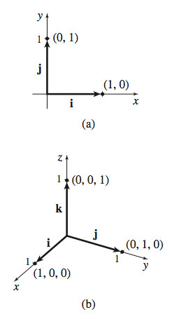
In space, the standard basis vectors are \bbox[5px, border:1px solid black, #F9F7ED]{ \mathbf{i} = \langle 1,0,0\rangle\qquad \mathbf{j} = \langle 0,1,0\rangle\qquad \mathbf{k} = \left\langle 0,0,1\right\rangle }
See Figure 29(a) and 29(b).
THEOREM Writing a Vector in Terms of Standard Basis Vectors
Every vector \mathbf{v} = (v_{1},v_{2}\ ) in the plane can be written in terms of the standard basis vectors \mathbf{i} and \mathbf{j} as \bbox[5px, border:1px solid black, #F9F7ED]{ \mathbf{v} = v_{1}\mathbf{i} + v_{2} \mathbf{j}}
Every vector \mathbf{v} = \langle v_{1}, v_{2}, v_{3}\rangle in space can be written in terms of the standard basis vectors \mathbf{i}, \mathbf{j}, and \mathbf{k} as \bbox[5px, border:1px solid black, #F9F7ED]{ \mathbf{v} = v_{1} \mathbf{i} + v_{2} \mathbf{j} + v_{3} \mathbf{k}}
The proof for vectors in the plane follows. The proof for vectors in space is left as an exercise (Problem 109).
Proof
\mathbf{v} = \left\langle v_{1}, v_{2}\right\rangle = \left\langle v_{1}, 0\right\rangle + \left\langle 0, v_{2}\right\rangle = v_{1} \left\langle 1, 0\right\rangle + v_{2} \left\langle 0, 1\right\rangle = v_{1} \mathbf{i} + v_{2} \mathbf{j}
EXAMPLE 6Writing a Vector Using Standard Basis Vectors
- (a) \langle 4, 3\rangle = 4 \mathbf{i} + 3 \mathbf{j}
- (b) \langle 2, -3\rangle = \dot{2}\mathbf{i} + (-3\dot{)}\mathbf{j} = 2 \mathbf{i} - 3 \mathbf{j}
- (c) \langle 1, -3, 2\rangle = \mathbf{i}-3 \mathbf{j} + 2 \mathbf{k}
- (d) \langle 0, 3, 4\rangle = 0 \mathbf{i} + 3 \mathbf{j} + 4 \mathbf{k} = 3 \mathbf{j} + 4 \mathbf{k}
NOW WORK
EXAMPLE 7Working with Standard Basis Vectors
- (a) If \mathbf{v} = 2 \mathbf{i} - 3 \mathbf{j} and \mathbf{w} = -\mathbf{i} + 2 \mathbf{j}, find 4\mathbf{v}-\mathbf{w}.
- (b) If \mathbf{v} = 2\mathbf{i} + 3 \mathbf{j} -\mathbf{k} and \mathbf{w} = -\mathbf{i}-2\mathbf{j}+4\mathbf{k}, find 2 \mathbf{v}-3 \mathbf{w}.
Solution
(a) \begin{align*} 4\mathbf{v} - \mathbf{w} = 4 (2 \mathbf{i} - 3 \mathbf{j}) - (-\mathbf{i} + 2 \mathbf{j}) = (8 \mathbf{i} - 12 \mathbf{j}) + (\mathbf{i} - 2 \mathbf{j}) = 9 \mathbf{i} - 14 \mathbf{j} \end{align*}
(b) \begin{align*} 2 \mathbf{v} - 3 \mathbf{w} &= 2(2 \mathbf{i} + 3 \mathbf{j} - \mathbf{k}) - 3(-\mathbf{i} - 2 \mathbf{j} + 4 \mathbf{k}) \\ & =(4 \mathbf{i} + 6 \mathbf{j} - 2 \mathbf{k}) + (3 \mathbf{i} + 6 \mathbf{j} - 12 \mathbf{k}) = 7 \mathbf{i} + 12 \mathbf{j} - 14 \mathbf{k} \end{align*}
NOW WORK
5 Find a Vector in the Plane from Its Direction and MagnitudePrinted Page 709
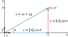
Often a vector is described by its magnitude and direction, rather than by its components. For example, a weather report warning of 40 \,\rm{mi/h} southwesterly winds (from the southwest) describes a velocity vector, but to work with it requires finding its components. A nonzero vector \mathbf{ v} in the plane can be described by specifying the angle \theta, 0 \leq \theta < 2 \pi, between \mathbf{v} and the positive x-axis, which gives its direction, and by specifying its magnitude \Vert \mathbf{v} \Vert. See Figure 30. If \mathbf{v} = x\mathbf{i} + y\mathbf{j}, then x = \Vert \mathbf{v}\Vert \cos \theta and y = \Vert \mathbf{v} \Vert \sin \theta. So, \mathbf{v} = \Vert \mathbf{v}\Vert \cos \theta \mathbf{i} + \Vert \mathbf{v}\Vert \sin \theta \mathbf{j} = \Vert \mathbf{v}\Vert (\cos \theta \,\mathbf{i} + \sin \theta \mathbf{j}).
THEOREM
If \mathbf{v} is a nonzero vector, and if \theta is the angle between \mathbf{v} and the positive x-axis, then \bbox[5px, border:1px solid black, #F9F7ED]{ \mathbf{v}=\left\Vert \mathbf{v}\right\Vert \left( \cos \theta \,\mathbf{i}+\sin \theta \,\mathbf{j}\right)}
710
NOTE
Wind direction is measured from where it blows.
EXAMPLE 8Using Standard Basis Vectors to Model a Problem
An airplane has an air speed of 400 km/h and is headed east. There is a northwesterly wind of 80 km/h. (Northwesterly winds blow toward the southeast.)
- (a) Find a vector representing the velocity of the airplane in the air.
- (b) Find a vector representing the wind velocity.
- (c) Find a vector representing the velocity of the airplane relative to the ground.
- (d) Find the true speed of the airplane.
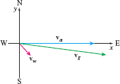
Solution We use a two-dimensional coordinate system with the direction north along the positive y-axis. Then the direction east is along the positive x-axis.
Using a scale of 1~\hbox{unit} = 1 km/h, define \begin{eqnarray*} \mathbf{v}_{\mathrm{a}} &=& \hbox{Velocity of the airplane in the air}\\[2pt] \mathbf{v}_{\mathrm{w}} &=& \hbox{Velocity of the wind}\\[2pt] \mathbf{v}_{\mathrm{g}} &=& \hbox{Velocity of the airplane relative to the ground} \end{eqnarray*}
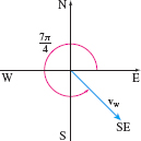
Figure 31 shows the vectors \mathbf{v}_{a}, \mathbf{v}_{w}, \mathbf{v}_{g}.
- (a) The vector \mathbf{v}_{\rm{a}} has magnitude 400 and direction \mathbf{i}, so \mathbf{v}_{\mathrm{a}} = 400i.
- (b) The vector \mathbf{v}_{\mathrm{w}} has magnitude 80 and makes an angle of \dfrac{7\pi}{4} with the positive x-axis, as shown in Figure 32. Since the magnitude of \mathbf{v}_{\rm{w}} is 80, \mathbf{v}_{\rm{w}} = 80\left(\cos \dfrac{7\pi}{4}\mathbf{i} + \sin \dfrac{7\pi}{4}\mathbf{j}\right) = 80 \left(\dfrac{\sqrt{2}}{2}\mathbf{i} - \dfrac{\sqrt{2}}{2}\mathbf{j}\right) = 40\sqrt{2}\mathbf{i} - 40\sqrt{2}\mathbf{j}
- (c) The velocity \mathbf{v}_{\mathrm{g}} of the airplane relative to the ground is the resultant of \mathbf{v}_{\rm{a }} and \mathbf{v}_{\rm{w}}. \mathbf{v}_{\mathrm{g}} = \mathbf{v}_{\mathrm{a}} + \mathbf{v}_{\mathrm{w}} = 400\ \mathbf{i} + \left[ 40\sqrt{2} \mathbf{i} - 40\sqrt{2} \mathbf{j}\right] = (400 + 40\sqrt{2}) \mathbf{i} - 40\sqrt{2} \mathbf{j}
- (d) The true speed of the airplane is the magnitude of the vector \mathbf{v}_{\mathrm{g}}. \left\Vert \mathbf{v}_{\mathrm{g}}\right\Vert =\sqrt{(400 + 40\sqrt{2})^{2} + (40\sqrt{2})^{2}}\approx 460.060
The true speed of the airplane is approximately 460.060 \,\rm{km/h}.
The direction of the airplane relative to the ground can be found using trigonometry, but we provide an easier method in the next section.
NOW WORK
When multiple forces \mathbf{F}_{1}, \mathbf{F}_{2}, \ldots, \mathbf{F} _{n} simultaneously act on an object, the vector sum \mathbf{F}_{1}+ \mathbf{F}_{2}+ \cdots + \mathbf{F}_{n} is the resultant force. The resultant force produces the same effect on the object as that obtained when each of the forces \mathbf{F}_{1}, \mathbf{F}_{2}, \ldots, \mathbf{F}_{n} acts on the same object at the same time. An object is in static equilibrium if the object is at rest and the resultant force is \mathbf{0}.
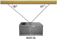
EXAMPLE 9Finding the Tension in Cable
A commercial air conditioner weighing 8600 lb is suspended from two cables, as shown in Figure 33. What is the tension in each cable?
711
Solution We represent the cables and the air conditioner with a force diagram, as shown in Figure 34.
The tension in each cable is the magnitude of \Vert\mathbf{F}_{1}\Vert and \Vert\mathbf{F}_{2}\Vert, respectively. The weight of the air conditioner is \Vert\mathbf{F}_{3}\Vert = 8600~\text{lb}. \begin{eqnarray*} \mathbf{F}_{1} &=& \Vert\mathbf{F}_{1}\Vert \left( \cos 45^{\circ}\mathbf{i} + \sin 45^{\circ}\mathbf{j}\right) = \Vert\mathbf{F}_{1}\Vert \left(\dfrac{\sqrt{2}}{2} \mathbf{i} + \dfrac{\sqrt{2}}{2} \mathbf{j}\right) \\[4pt] \mathbf{F}_{2} &=& \Vert \mathbf{F}_{2}\Vert \left(\cos 140^{\circ} \mathbf{i} + \sin 140^{\circ} \mathbf{j}\right) \\[4pt] \mathbf{F}_{3} &=& -8600 \mathbf{j} \end{eqnarray*}
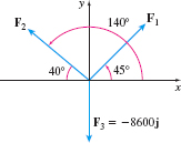
For the air conditioner to be in static equilibrium, the sum of the forces acting on it must equal \mathbf{0}. That is, \begin{eqnarray*} \mathbf{F}_{1} + \mathbf{F}_{2} + \mathbf{F}_{3} &=& \left(\dfrac{\sqrt{2}}{2} \Vert\mathbf{F}_{1}\Vert \mathbf{i} + \dfrac{\sqrt{2}}{2} \Vert\mathbf{F}_{1}\Vert \mathbf{j}\right)\\[6pt] &&+ \left(\cos 140^{\circ} \Vert\mathbf{F}_{2}\Vert \mathbf{i} + \sin 140^{\circ} \Vert\mathbf{F}_{2}\Vert \mathbf{j}\right) -8600\mathbf{j} = \mathbf{0} \end{eqnarray*}
Since both the \mathbf{i} and \mathbf{j} components equal 0, we have a system of two equations: \begin{equation*} \left\{ \begin{array}{rcl@{\hspace*{5pc}}r@{}} \dfrac{\sqrt{2}}{2}\Vert\mathbf{F}_{1}\Vert + \cos 140^{\circ} \Vert\mathbf{F}_{2}\Vert &=& 0 & \hbox{(1)} \\ \dfrac{\sqrt{2}}{2}\Vert \mathbf{F}_{1}\Vert + \sin 140^{\circ} \Vert\mathbf{F}_{2}\Vert -8600 &=& 0 & \hbox{(2)} \end{array} \right. \end{equation*}
We solve equation (1) for \left\Vert \mathbf{F}_{1}\right\Vert: \begin{equation*} \Vert\mathbf{F}_{1}\Vert = -\dfrac{2\cos 140^{\circ} \Vert\mathbf{F}_{2}\Vert}{\sqrt{2}} \tag{3} \end{equation*}
and substitute the result into equation (2). \begin{eqnarray*} \dfrac{\sqrt{2}}{2}\left(-\dfrac{2\cos 140^{\circ} \Vert\mathbf{F}_{2}\Vert}{\sqrt{2}}\right) + \sin 140^{\circ} \Vert\mathbf{F}_{2}\Vert -8600 &=& 0 \\[4pt] \left[-\cos 140^{\circ} + \sin 140^{\circ} \right] \Vert\mathbf{F}_{2}\Vert &=& 8600 \\[4pt] \Vert \mathbf{F}_{2}\Vert &=& \dfrac{8600}{\sin 140^{\circ} - \cos 140^{\circ}}\approx 6104 \end{eqnarray*}
Then from (3) \begin{equation*} \Vert\mathbf{F}_{1}\Vert = -\dfrac{2\cos 140^{\circ} \Vt\mathbf{F}_{2}\Vert}{\sqrt{2}}\approx -\dfrac{2\cos 140^{\circ}}{\sqrt{2}}(6104) \approx 6613 \end{equation*}
The left cable has a tension of approximately 6104~\text{lb} and the right cable has a tension of approximately 6613~\text{lb}.
NOW WORK
Vectors in n Dimensions
Printed Page 711
In a space of n dimensions, the rectangular coordinates of a point are given by an ordered n-tuple (v_{1}, v_{2},\ldots,v_{n}) of real numbers. A vector \mathbf{v} in n-space whose initial point is at the origin and whose terminal point is at (v_{1},v_{2},\ldots,v_{n}) is defined as \bbox[5px, border:1px solid black, #F9F7ED]{ \mathbf{v} = \langle v_{1},v_{2},\ldots,v_{n}\rangle}
712
where the numbers v_{1}, v_{2}, \ldots , v_{n} are the components of \mathbf{v}. In n-space there are n coordinate axes and, along each positive axis, a standard basis vector is defined as follows: \bbox[5px, border:1px solid black, #F9F7ED]{ \mathbf{e}_{1} = \langle 1,0,\ldots, 0\rangle,\quad \mathbf{e}_{2} = \langle 0,1,\ldots,0\rangle,\quad \ldots, \quad \mathbf{e}_{n} = \langle 0,0,\ldots,1\rangle}
Any vector \mathbf{v} = \langle v_{1},v_{2},\ldots,v_{n}\rangle in n-space can be written in terms of the standard basis vectors \mathbf{e}_{1}, \mathbf{e}_{2},\ldots, \mathbf{e}_{n} as \bbox[5px, border:1px solid black, #F9F7ED]{ \mathbf{v} = v_{1} \mathbf{e}_{1} + v_{2} \mathbf{e}_{2} + \cdots + v_{n} \mathbf{e}_{n}}
We add two vectors in n-space by adding respective components. The scalar multiple a \mathbf{v} of a vector is found by multiplying each component by the scalar a. The magnitude of the vector \mathbf{v} = v_{1} \mathbf{e} _{1} + v_{2} \mathbf{e}_{2} + \cdots + v_{n} \mathbf{e}_{n} is \Vert \mathbf{v}\Vert = \sqrt{v_{1}^{2} + v_{2}^{2} + \cdots + v_{n}^{2}}.