13.3 Extrema of Functions of Two VariablesPrinted Page 879
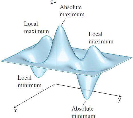
An important application of the derivative of a function of a single variable is to identify local extrema and absolute extrema. In a similar way, partial derivatives are used to identify the extrema of a function of several variables. We begin with the definitions of the local maximum and the local minimum of a function z=f(x,y) of two variables. Compare these definitions to those given for a function f of a single variable.
NEED TO REVIEW?
Local extrema and absolute extrema of a function of a single variable are discussed in Section 4.2, pp. 263-272.
DEFINITION Local Maximum, Local Minimum
Let z=f(x,y) be a function with domain D and let (x0,y0) be an interior point of D. Then f has a local maximum at (x0,y0) if f(x0,y0)≥f(x,y)
for all points (x,y) within some disk centered at (x0,y0). The number f(x0,y0) is called a local maximum value.
The function f has a local minimum at (x0,y0) if f(x0,y0)≤f(x,y)
for all points (x,y) within some disk centered at (x0,y0). The number f(x0,y0) is called a local minimum value.
Collectively, the local maxima and local minima of f are called local extrema.
DEFINITION Absolute Maximum, Absolute Minimum
Let z=f(x,y) be a function with domain D. If there is a point (x0,y0) in D for which f(x0,y0)≥f(x,y) for all (x,y) in D, then f has an absolute maximum at (x0,y0) and f(x0,y0) is called the absolute maximum value of f on D.
If there is a point (x0,y0) in D for which f(x0,y0)≤f(x,y) for all (x,y) in D, then f has an absolute minimum at (x0,y0) and f(x0,y0) is the absolute minimum value of f on D.
The absolute maximum and absolute minimum of f are called the absolute extrema of the function.
880
Figure 12 illustrates these definitions. Notice that the tangent plane at each local extremum is parallel to the xy-plane.
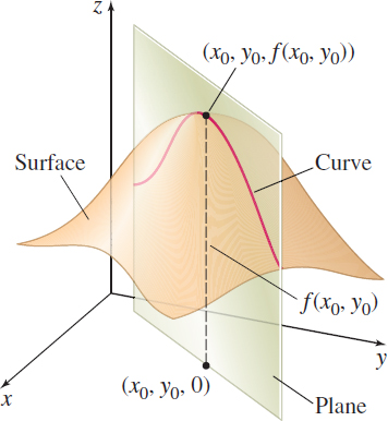
Let z=f(x,y) be a function of two variables that is defined and continuous on an open set D. Suppose f has a local maximum at the point (x0,y0) in D. Then the curve that results from the intersection of the surface z=f(x,y) and any plane through (x0,y0,0) that is perpendicular to the xy-plane will have a local maximum at (x0,y0). See Figure 13.
In particular, the curve that results from intersecting z=f(x,y) with the plane x=x0 has this property. This means that if fy(x0,y0) exists, then fy(x0,y0)=0. By a similar argument, if the surface z=f(x,y) is intersected by the plane y=y0, then the curve that results has a local maximum at (x0,y0), and if fx(x0,y0) exists, then fx(x0,y0)=0.
THEOREM A Necessary Condition for Local Extrema
Let z=f(x,y) be a function of two variables that is defined and continuous on an open set containing the point (x0,y0). Suppose fx and fy each exist at (x0,y0). If f has a local extremum at (x0,y0), then {\bbox[#FAF8ED]{\bbox[5px, border:1px solid black, #F9F7ED]{ f_{x}(x_{0},y_{0})=0\qquad \hbox{and} \qquad f_{y}(x_{0},y_{0})=0 }}}
The theorem asserts that if a function f has local extrema, they will occur at those points at which the partial derivatives of f exist and equal 0. Further, if f has a local extremum at ( x_{0},y_{0}) , then the tangent plane to f at ( x_{0},y_{0}) is z-z_{0}=0, where z_{0}=f( x_{0},y_{0}) . That is, the tangent plane is parallel to the xy-plane.
It can also happen that the local extrema of a function occur at points at which one or both of the partial derivatives fail to exist. For example, the cone z=\sqrt{x^2+y^2} has a local minimum at (0,0) where both f_x and f_y do not exist.
DEFINITION Critical Point
Let z=f(x,y) be a function of two variables whose domain is an open set D containing the point (x_{0},y_{0}). The point (x_{0},y_{0}) is a critical point of f if:
- f_{x}(x_{0},y_{0})=f_{y}(x_{0},y_{0})=0.
- either f_{x}(x_{0},y_{0}) or f_{y}(x_{0},y_{0}) does not exist.
Using the definition of critical point, the necessary condition for local extrema is restated.
THEOREM A Necessary Condition for Local Extrema
Let z=f(x,y) be a function of two variables whose domain is an open set D. If f has a local extremum at (x_{0},y_{0}), then (x_{0},y_{0}) is a critical point of f.
1 Find Critical PointsPrinted Page 880
EXAMPLE 1Finding Critical Points
Find the critical points of the function z=f(x,y)=x^{2}+y^{2}-2x+4y
Solution The partial derivatives of f are f_{x}=2x-2\qquad \hbox{and} \qquad f_{y}=2y+4
881
Since both partial derivatives exist for all x and y, the critical points of f satisfy the system of equations \left\{\begin{array}{l} 2x-2=0\\[3pt] 2y+4=0 \end{array}\right.
Solving the system simultaneously, we find that the only critical point is (1,-2) .
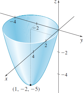
z=f(x,y)=x^{2}+y^{2}-2x+4y
has a local minimum at (1,-2).
We can determine whether the function in Example 1 has a local maximum or a local minimum or neither at the critical point by rewriting the function in a simpler form. \begin{array}{rcl@{\qquad}l} z &=&x^{2}+y^{2}-2x+4y & {\color{#0066A7}{\hbox{\(z=f(x,y)\).}}}\\ z &=&( x^{2}-2x+1) +( y^{2}+4y+4) -5 & {\color{#0066A7}{\hbox{Complete the squares.}}}\\ z &=&( x-1) ^{2}+( y+2) ^{2}-5 & {\color{#0066A7}{\hbox{Factor.}}} \end{array}
Since z\geq -5, there is a local minimum at ( 1,-2); the local minimum value is -5. In fact, the absolute minimum occurs at the point (1,-2) and the absolute minimum value is -5. See Figure 14.
NOW WORK
As with functions of one variable, it is possible for a function z= f( x,y) to have a critical point at ( x_{0},y_{0}) , but no local extremum at ( x_{0},y_{0}) .
EXAMPLE 2Finding Critical Points
Consider the hyperbolic paraboloid defined by the equation z=f(x,y)=y^{2}-x^{2}. Show that (0,0) is the only critical point of f, but that f has neither a local maximum nor a local minimum at (0,0).
Solution The partial derivatives of f are f_{x}(x,y)=-2x\qquad \hbox{and} \qquad f_{y}(x,y)=2y
At ( 0,0) , both partial derivatives equal 0, so (0,0) is the only critical point.
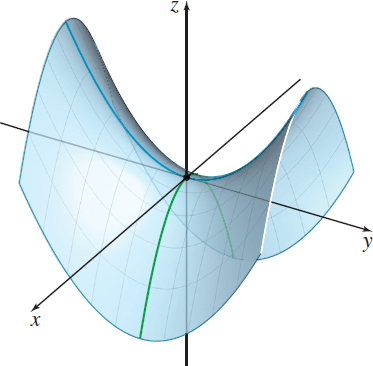
See Figure 15. If we consider the values of f(x,0)=-x^{2}, the function attains a maximum value of 0 at the origin. However, if we consider the values of f(0,y)=y^{2}, the function attains a minimum value at the origin. In other words, at the critical point (0,0), the function appears to have a maximum when viewed in one direction and to have a minimum when viewed in another direction. As a result, z=f(x,y)=y^{2}-x^{2} has neither a maximum nor a minimum at (0,0).
Example 2 and Figure 15 help explain the next definition.
DEFINITION Saddle Point
A point (x_{0},y_{0},f(x_{0},y_{0})) is called a saddle point of z=f( x,y) if both f_{x}(x_{0},y_{0})=0 and f_{y}(x_{0},y_{0})=0, but f does not have a local extremum at (x_{0},y_{0}).
In Examples 1 and 2, we used algebraic and/or geometric arguments to determine whether a critical point resulted in a local maximum, a local minimum, or a saddle point. For most functions, such arguments cannot be used. The following test, which is stated without a proof, provides an analytic method to determine the nature of critical points. The test is analogous to the Second Derivative Test for functions of one variable. A proof of the theorem can be found in texts on advanced calculus.
882
NOTE
The expression AC-B^{2}= f_{xx} f_{yy}-f_{xy}^{2} is also called the discriminant or Hessian of f. It is often written as the determinant AC-B^{2} =f_{xx} f_{yy} -f_{xy}^{2} = \left\vert \begin{array}{c@{\quad}c} f_{xx} & f_{xy} \\[3pt] f_{xy} & f_{yy} \end{array} \right\vert
THEOREM Second Partial Derivative Test for Local Extrema
Let z=f(x,y) be a function of two variables for which the first- and second-order partial derivatives are continuous in some disk containing the point (x_{0},y_{0}). Suppose f_{x}(x_{0},y_{0})=0 and f_{y}(x_{0},y_{0})=0. Let A=f_{xx}(x_{0},y_{0})\qquad B=f_{xy}(x_{0},y_{0}) \qquad C=f_{yy}(x_{0},y_{0})
- If AC-B^{2}>0 and A>0, then f has a local minimum at (x_{0},y_{0}).
- If AC-B^{2}>0 and A<0, then f has a local maximum at (x_{0},y_{0}).
- If AC-B^{2}<0, then f has a saddle point at (x_{0},y_{0}).
- If AC-B^{2}=0, then the test gives no information.
2 Use the Second Partial Derivative TestPrinted Page 882
EXAMPLE 3Using the Second Partial Derivative Test
Find all local maxima, local minima, and saddle points for z=f(x,y)=x^{2}+xy+y^{2}-6x+6
Solution The critical points of f are solutions of the system of equations \left\{ \begin{array}{rcll} f_{x}(x,y)&=&2x+y-6&=0 \\[3pt] f_{y}(x,y)&=&x+2y &=0 \end{array} \right.
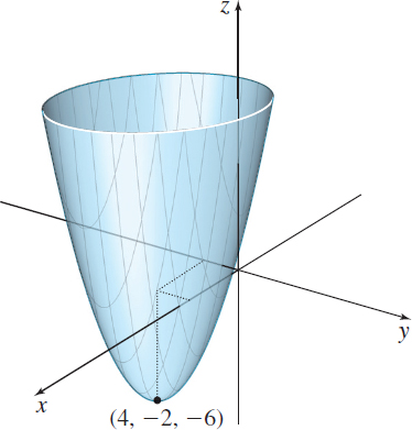
The only solution is x=4 and y=-2, so (4,-2) is the only critical point.
The second-order partial derivatives of f are f_{xx}(x,y)=2\qquad f_{xy}(x,y)=f_{yx}( x,y) =1 \qquad f_{yy}(x,y)=2
The function f meets the requirements of the Second Partial Derivative test at the critical point (4,-2). Now A=f_{xx}(4,-2)=2\qquad B=f_{xy}(4,-2)=1 \qquad C=f_{yy}(4,-2)=2 AC-B^{2}=( 2) ( 2) -1^{2}=3>0
Since AC-B^{2}>0 and A= f_{xx}(4,-2)=2>0, the Second Partial Derivative Test guarantees that f has a local minimum at (4,-2). The local minimum value is z=f(4,-2)=-6. See Figure 16.
NOW WORK
NOTE
To find the critical points of a function z=f(x,y) we must solve the system of equations f_{x} =0 and f_{y} =0. If the system is nonlinear, no general method of solution is available and a CAS is generally used. If solving by hand, care must be taken because extraneous roots are sometimes introduced.
EXAMPLE 4Using the Second Partial Derivative Test
Find all local maxima, local minima, and saddle points for z=f(x,y)=x^{3}+y^{2}+2xy-4x-3y+5
Solution The critical points are the solutions of the system of equations \left\{ \begin{array}{rcll} f_{x}(x,y)&=&3x^{2}+2y-4&=0 \\[3pt] f_{y}(x,y)&=&2y+2x-3&=0 \end{array}\right.
We solve the system using substitution. Solving for y in f_{y}(x,y)=0, we obtain y=\dfrac{1}{2}(3-2x). Then if we substitute for y in f_{x}(x,y)=0, the result is \begin{eqnarray*} 3x^{2}+2\,\left[ \dfrac{1}{2}(3-2x)\right] -4& =0 \\[4pt] 3x^{2}-2x-1& =0 \\[4pt] (3x+1)(x-1)& =0 \\[4pt] x=-\dfrac{1}{3}\qquad \hbox{or }\qquad x& =1 \end{eqnarray*}
883
When x=-\dfrac{1}{3}, then y=\dfrac{1}{2}(3-2x)=\dfrac{1}{2}\left( 3+ \dfrac{2}{3}\right) =\dfrac{11}{6}.
When x=1, then y=\dfrac{1}{2}(3-2x)=\dfrac{1}{2}.
The critical points are \left( -\dfrac{1}{3},\dfrac{11}{6}\right) and \left( 1,\dfrac{1}{2}\right) .
The second-order partial derivatives of f are f_{xx}(x,y)=6x\qquad f_{xy}(x,y)=2\qquad f_{yy}(x,y)=2
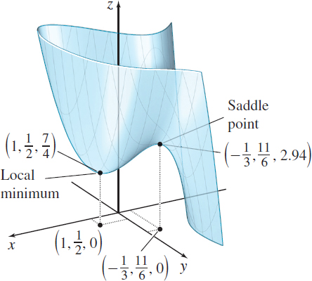
The function f satisfies the requirements of the Second Partial Derivative test at each critical point. At \left( -\dfrac{1}{3},\dfrac{11}{6}\right) , \begin{eqnarray*} &A=f_{xx}\left( -\dfrac{1}{3},\dfrac{11}{6}\right) =-2\qquad B=f_{xy}\left( -\dfrac{1}{3},\dfrac{11}{6}\right) =2\qquad C=f_{yy}\left( -\dfrac{1}{3},\dfrac{11}{6}\right) =2&\\[4pt] &AC-B^{2}=-4-4=-8<0& \end{eqnarray*}
So, \left( -\dfrac{1}{3},\dfrac{11}{6},\dfrac{317}{108}\right) is a saddle point of f. At \left( 1,\dfrac{1}{2}\right) , A=f_{xx}\left( 1,\dfrac{1}{2}\right) =6\qquad B=f_{xy}\left( 1,\dfrac{1}{2}\right) =2\qquad C=f_{yy}\left( 1,\dfrac{1}{2}\right)=2
Since AC-B^{2}=8>0, f has a local minimum at \left( 1,\dfrac{1}{2}\right) , where f\left( 1,\dfrac{1}{2}\right) =\dfrac{7}{4}
A graph of z=f(x,y)=x^{3}+y^{2}+2xy-4x-3y+5 is shown in Figure 17.
NOW WORK
3 Find the Absolute Extrema of a Function of Two VariablesPrinted Page 883
For a function f of one variable, the Extreme Value Theorem states that if f is continuous on a closed interval [a,b], then f has an absolute maximum value and an absolute minimum value on that interval. For functions of two variables, there is a similar theorem. But first we need to define the set in the plane that is analogous to a closed interval on the real line.
NEED TO REVIEW?
Open and closed sets are discussed in Section 12.2, p. 825.
Recall that a set D is closed if it contains all its boundary points. We say that D is bounded if D can be enclosed by some disk (if D is in the plane) or by some ball (if D is in space). With this definition, we can state the following two-variable version of the Extreme Value Theorem:
THEOREM Extreme Value Theorem for Functions of Two Variables
Let z=f(x,y) be a function of two variables. If f is continuous on a closed, bounded set D, then f has an absolute maximum and an absolute minimum on D.
To find the absolute extrema of a function meeting the criteria of the Extreme Value Theorem for Functions of Two Variables, we note that if f has an extreme value at (x_{0},y_{0}), then (x_{0},y_{0}) either is a critical point of f or is a boundary point of D. As a result, we have the following test:
884
THEOREM Test for Absolute Maximum and Absolute Minimum
Let z=f(x,y) be a function of two variables defined on a closed, bounded set D. If f is continuous on D, then the absolute maximum value and the absolute minimum value of f are, respectively, the largest and smallest values found among the following:
- The values of f at the critical points of f in D
- The values of f on the boundary of D
EXAMPLE 5Finding Absolute Extrema
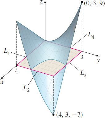
Find the absolute maximum and the absolute minimum of \begin{equation*} z=f(x,y)=2x-2xy+y^{2} \end{equation*}
whose domain is the region defined by 0\leq x\leq 4 and 0\leq y\leq 3.
Solution The function f is continuous on its domain, which is a closed, bounded set. Then the Extreme Value Theorem guarantees that f has an absolute maximum and an absolute minimum on its domain. To find them, we first find the critical points of f, namely the solutions of the system of equations \left\{\begin{array}{l} f_{x}(x,y)=2-2y=0\\ f_{y}(x,y)=-2x+2y=0 \end{array}\right.
Solving the system of equations, we find that the only critical point is (1,1). The value of f at (1,1) is f(1,1)=2(1) -2(1) (1) +1^{2}=1
The domain of f is the set 0\leq x \leq 4, 0\leq y\leq 3. The boundary of the domain of f consists of the four line segments L_1, L_2, L_3, and L_4 shown in Figure 18. We evaluate f on each line segment.
On \boldsymbol L_{\bf 1}: x is in the interval \left[ 0,4\right] and y=0. The function f(x,y)=f(x,0)=2x is increasing on 0\leq x\leq 4, so its extreme values occur at the endpoints 0 and 4. \hbox{At }x=0, f(0,0)=0\qquad \hbox{and} \qquad \hbox{at}\ x=4, f(4,0)=8
On \boldsymbol L_{\bf 2}: x=4 and y is in the interval [0,3] . The function f(x,y)=f(4,y)= 8-8y+y^{2}. To find the extreme values of f on [0,3] , we begin by finding the critical number(s) of the function g(y) =8-8y+y^{2}. That is, we find where g' (y) =0. \begin{eqnarray*} g' (y) &=&-8+2y=0 \\[3pt] y &=&4 \end{eqnarray*}
Since 4 is not in the interval [0,3] , the extreme values occur at the endpoints 0 and 3. \hbox{At }y=0\hbox{, }\ f(4,0)=8\qquad \hbox{and} \qquad \hbox{at}y=3,\hbox{ }f(4,3)=-7
On \boldsymbol L_{\bf 3}: x is in the interval [ 0,4] and y=3. The function f(x,y)=f(x,3)= 2x-6x+9=-4x+9 is decreasing on 0\leq x\leq 4, so its extreme values occur at the endpoints 0 and 4. \hbox{At }x=0, f(0,3)=9\qquad \hbox{and} \qquad \hbox{at }x=4, f(4,3)=-7
On \boldsymbol L_{\bf 4}: x=0 and y is in the interval [0,3] . The function f(x,y)=f(0,y)=y^{2} is increasing on 0\leq y\leq 3, so its extreme values occur at the endpoints 0 and 3. \hbox{At }y=0, f(0,0)=0\qquad\hbox {and}\qquad \hbox{at }y=3,\hbox{ }f(0,3)=9
885
The values of f at the critical point (1,1) and at the extreme values on the boundary are
| Point | (1,1) | ( 0,0) | ( 4,0) | ( 4,3) | ( 0,3) |
| Value | 1 | 0 | 8 | -7 | 9 |
The absolute maximum value of f is f(0,3)=9; the absolute minimum value is f(4,3)=-7.
NOW WORK
EXAMPLE 6Finding Absolute Extrema
Find the absolute maximum and the absolute minimum of \begin{equation*} z=f( x,y) =x^{2}+y^{2}-2x+2y-5 \end{equation*}
whose domain is the disk x^{2}+y^{2}\leq 9.
Solution The function f is continuous on its domain, a closed, bounded set. The Extreme Value Theorem guarantees that f has an absolute maximum and an absolute minimum on its domain. To find them, we find the critical points of f, namely the solutions of the system of equations \left\{\begin{array}{l} f_{x}( x,y) =2x-2=0\\[3pt] f_{y}( x,y) =2y+2=0 \end{array}\right.
The only solution is x=1, y=-1, which is an interior point of the domain of f. The value of f at the critical point is f(1,-1) =-7.
The boundary of the domain of f is the circle x^{2}+y^{2}=9. We express the boundary using the parametric equations x=x(t) =3\,\cos t, y=y(t) =3\,\sin t, 0\leq t\leq 2\pi . Next we evaluate f on its boundary. \begin{eqnarray*} z=f( x,y) &=&f( 3\,\cos t,3\,\sin t)\\[4pt] &=&9\,\cos ^{2}t+9\,\sin^{2}t-6\,\cos t+6\,\sin t-5\\[4pt] &=&4-6\,\cos t+6\,\sin t \end{eqnarray*}
Now we find where \dfrac{dz}{dt}=0. \begin{eqnarray*} \dfrac{dz}{dt}&= & 6\,\sin t+6\,\cos t=0 \\[4pt] \tan t&=&-1 \\[4pt] t&=&\dfrac{3\pi }{4}\qquad\hbox{or}\qquad t=\dfrac{7\pi }{4} \end{eqnarray*}
At t=\dfrac{3\pi }{4}, the value of f is \begin{eqnarray*} f\left( 3\,\cos \dfrac{3\pi }{4},3\,\sin \dfrac{3\pi }{4}\right) &=&4-6\,\cos \dfrac{ 3\pi }{4}+6\,\sin \dfrac{3\pi }{4}=4-6\left( -\dfrac{\sqrt{2}}{2}\right) +6\left( \dfrac{\sqrt{2}}{2}\right)\\[4pt] &=&4+6\sqrt{2} \end{eqnarray*}

At t=\dfrac{7\pi }{4}, the value of f is \begin{eqnarray*} f\left( 3\,\cos \dfrac{7\pi }{4},3\,\sin \dfrac{7\pi }{4}\right) &=&4-6\,\cos \dfrac{ 7\pi }{4}+6\,\sin \dfrac{7\pi }{4}=4-6\left( \dfrac{\sqrt{2}}{2}\right) +6\left( -\dfrac{\sqrt{2}}{2}\right)\\[4pt] &=&4-6\sqrt{2} \end{eqnarray*}
886
The absolute maximum value of f is 4+6\sqrt{2}\approx 12. 485; the absolute minimum value of f is -7.
Figure 19 shows the graph of z=f( x,y) =x^{2}+y^{2}-2x+2y-5.
NOW WORK
4 Solve Optimization ProblemsPrinted Page 886
Now that we have the tools for finding the extrema of functions of two variables, we can investigate applied problems that involve optimization.
EXAMPLE 7Solving an Optimization Problem: Minimizing Resources Used
A manufacturer wants to make an open rectangular box of volume V=500 cubic centimeters (\rm{cm}^3) using the least possible amount of material. Find the dimensions of the box.
Solution Let x and y be the dimensions of the base of the box, and let z be the height of the box. Then V=500=xyz\,\rm{cm}^{3}\qquad x>0\quad y>0\quad z>0
The manufacturer wants to minimize the amount of material used, which equals the surface area S of the box. Since the box is open, S=xy+2xz+2yz
If we solve the equation 500=xyz for z and substitute z=\dfrac{500}{xy} into the formula for the surface area S of the box, we can express S as a function of two variables. S=S( x,y) =xy+2x\!\left( \dfrac{500}{xy}\right) +2y\left( \dfrac{500 }{xy}\right) =xy+\frac{1000}{y}+\frac{1000}{x}
This is the function to be minimized. The partial derivatives of S are S_{x}=y-\dfrac{1000}{x^{2}}\qquad \hbox{and} \qquad S_{y}=x-\dfrac{1000}{y^{2}}
Since x>0 and y>0, the critical points satisfy the system of equations \left\{\begin{array}{l} y-\dfrac{1000}{x^{2}}=0\\[3pt] x-\dfrac{1000}{y^{2}}=0 \end{array}\right.
Using substitution, we find x=y=1000^{1/3}=10
The second-order partial derivatives of S are \begin{eqnarray*} S_{xx}&=&\dfrac{\partial }{\partial x}\left( y-\dfrac{1000}{x^{2}}\right) =\dfrac{2000}{x^{3}}\qquad S_{xy}= \dfrac{\partial }{\partial x}\left(x-\dfrac{1000}{y^{2}}\right) =1\\[4pt] S_{yy}&=&\dfrac{\partial }{\partial y}\left( x-\dfrac{1000}{y^{2}}\right) =\dfrac{2000}{y^{3}} \end{eqnarray*}
At the critical point ( 10,10) , \begin{eqnarray*}\hspace{-1pc} &\hspace{-1.8pc}A=S_{xx}(10,10) =\dfrac{2000}{10^{3}}=2\qquad B=S_{xy}(10,10) =1\qquad C=S_{yy}(10,10) =\dfrac{2000}{10^{3}}=2 &\hspace{1.8pc}\\[4pt] &AC-B^{2}=3>0& \end{eqnarray*}
From the Second Partial Derivative Test, S has a local minimum at (10,10).
But, we want to know where S attains its absolute minimum. Since the physical properties of the problem require that the absolute minimum exists, the local minimum is also the absolute minimum. Consequently, the dimensions (in centimeters) of the open box of volume V=500\,\rm{cm}^{3} that uses the least amount of material are x=10\rm{cm}\qquad y=10\rm{cm}\qquad z=\dfrac{500}{100}=5\rm{cm}
887
In Example 7, the conditions of the Extreme Value Theorem for Functions of Two Variables were not met, since the domain of S is not bounded. Fortunately, in applied problems (such as Example 7), it is often possible to argue from physical or geometric properties that an absolute extremum must exist and that it must occur at one of the local extrema.
NOW WORK
EXAMPLE 8Solving an Optimization Problem: Maximizing Profit
The demand functions for two products are p=12-2x\qquad \hbox{and}\qquad q=20-y
where p and q are the respective prices (in thousands of dollars) of each product, and x and y are the respective amounts (in thousands of units) of each sold. Suppose the joint cost function is C( x,y) =x^{2}+2xy+2y^{2}
- (a) Find the revenue function and the profit function.
- (b) Determine the prices and amounts that will maximize profit.
- (c) What is the maximum profit?
Solution (a) Revenue is the amount of money brought in. That is, revenue is the product of price and quantity sold. The revenue function R is the sum of the revenues from each product. R( x,y) =xp+yq=x( 12-2x) +y( 20-y)
Profit is the difference between revenue and cost. The profit function P is \begin{eqnarray*} P( x,y) &=&R( x,y) -C( x,y) =[ x(12-2x) +y( 20-y) ] -[ x^{2}+2xy+2y^{2}] \\[3pt] &=&12x-2x^{2}+20y-y^{2}-x^{2}-2xy-2y^{2}\\[3pt] &=&-3x^{2}-3y^{2}-2xy+12x+20y \end{eqnarray*}
(b) The partial derivatives of P are \begin{eqnarray*} P_{x}( x,y) &=&\dfrac{\partial }{\partial x}(-3x^{2}-3y^{2}-2xy+12x+20y) =-6x-2y+12 \\[4pt] P_{y}( x,y) &=&\dfrac{\partial }{\partial y}(-3x^{2}-3y^{2}-2xy+12x+20y) =-6y-2x+20 \end{eqnarray*}
We find the critical points by solving the system of equations: \left\{ \begin{array}{l} -6x-2y+12=0 \\[3pt] -2x-6y+20=0 \end{array} \right.
We solve the first equation for y and substitute the result into the second equation. Since y=6-3x, then \begin{eqnarray*} -2x-6( 6-3x) +20 &=&0 \\ x &=&1 \end{eqnarray*}
and y=6-3(1) =3, so (1,3) is the only critical point.
The second-order partial derivatives are A=P_{xx}( x,y) =-6\qquad B=P_{xy}( x,y) =-2\qquad C=P_{yy}( x,y) =-6
888
At the critical point (1,3) , \begin{array}{@{\hspace*{-3.4pc}}l} P_{xx}(1,3) =-6<0 \qquad P_{xy}(1,3) =-2 \qquad P_{yy}(1,3) =-6 \qquad AC-B^{2}=36-4=32>0 \end{array}
From the Second Partial Derivative Test, P has a local maximum at (1,3).
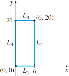
The domains of the demand functions p=12-2x and q=20-y are 0\leq x\leq 6 and 0\leq y\leq 20, respectively. Since the domain of the profit function P is 0\leq x\leq 6, 0\leq y\leq 20, the domain is closed and bounded, so a maximum profit exists. From the test for absolute maximum and absolute minimum, the maximum profit is found at a critical point or on the boundary of the domain.
Figure 20 shows the boundary of the profit function P and Table 1 gives the maximum value of P on its boundary and at the critical point (1,3).
| Maximum \bf P | ||
|---|---|---|
| L_{1}:\quad 0\le x \le 6, y=0 | P(x,0)= -3x^{2}+12x | P(2,0)=12 |
| L_{2}:\quad x=6, x \le y \le 20 | P(6,y)= -3y^{2}+8y -36 | P(6,y)<0 |
| L_{3}:\quad 0\le x \le 6, y= 20 | P(x,20)= -3x^{2}-28x -800 | P(x,20)<0 |
| L_{4}:\quad x=0, 0 \le y \le 20 | P(0,y)= -3y^{2}+20y | P(0,\frac{10}{3}) =33.33 |
| Critical point (1, 3): | P(1,3) =36 |
We conclude that by selling 1000 units of product x for the price p=12-2(1) =10 thousand dollars and 3000 units of product y for the price q=20-3=17 thousand dollars, the profit is maximized.
(c) The maximum profit is P(1,3) =$ 36,000.