7.6 Integration Using Numerical TechniquesPrinted Page 508
OBJECTIVES
When you finish this section, you should be able to:
Most of the functions we have encountered so far belong to the class known as elementary functions. These functions include polynomial, exponential, logarithm, trigonometric, inverse trigonometric, hyperbolic, and inverse hyperbolic functions, as well as functions formed by combining one or more of these functions using addition, subtraction, multiplication, division, or composition.
We have found that the derivatives f′, f′′, and so on, of an elementary function f are also elementary functions. The integral of an elementary function ∫f(x)dx, however, is not always an elementary function. Some examples of integrals of elementary functions that cannot be written in terms of elementary functions are \bbox[5px, border:1px solid black, #F9F7ED]{ \begin{array}{l@{\qquad}l@{\qquad}l@{\qquad}l@{\qquad}l@{}} \int e^{x^{2}}\,dx & \int e^{-x^{2}}\,dx & \int \dfrac{\sin x}{x}dx \\ \int \dfrac{\cos x}{x}dx & \int \dfrac{e^{x}\,dx}{x} & \int \dfrac{dx}{\sqrt{1-x^{3}}} \end{array} }
Recall that to find a definite integral using the Fundamental Theorem of Calculus requires an antiderivative of the integrand f. When it is not possible to express an antiderivative of f in terms of elementary functions, or when the integrand f is defined by a table of data or by a graph, the Fundamental Theorem is not useful. In such situations, there are numerical techniques we can use to approximate the definite integral.
In Chapter 5 we used Riemann sums to approximate definite integrals. Two other commonly used numerical techniques to approximate integrals are the Trapezoidal Rule and Simpson’s Rule. A fourth method, based on series, is discussed in Chapter 8.
1 Approximate an Integral Using the Trapezoidal RulePrinted Page 508
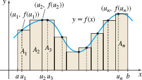
As we learned in Section 5.2, if a function f is nonnegative and continuous on an interval [a,b] , then the area A under the graph of f from a to b equals the definite integral \int_{a}^{b}f( x)\,dx. We can approximate A by partitioning [a,b] into n subintervals, each of width \Delta x=\dfrac{b-a }{n}; choosing a number u_{i} from each subinterval [x_{i-1},x_{i}], i=1,2,\ldots ,n; and forming n rectangles of height f(u_{i}) and width \Delta x. The sum of the areas of these rectangles approximates the integral \int_{a}^{b}f( x)\, dx. See Figure 11.
509
The Trapezoidal Rule approximates the definite integral \int_{a}^{b}f( x)\, dx by replacing the rectangles with trapezoids. Then the area A under the graph of f from a to b, \int_{a}^{b}f( x) \,dx, is approximated by the sum of the areas of these trapezoids.
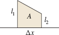
RECALL
The area A of a trapezoid with width \Delta x and parallel heights l_{1} and l_{2} is A =\dfrac{1}{2}(l_{1}+l_{2}) \Delta x.
The Trapezoidal Rule
If a function f is continuous on the closed interval [a,\,b ], then \bbox[5px, border:1px solid black, #F9F7ED]{ \int_{a}^{b}f(x)\,dx\approx \dfrac{b-a}{2n}\,\left[f(x_{0})+2f(x_{1})+2f(x_{2})+\cdots +2f(x_{n-1})+f(x_{n}) \right] }
where the closed interval [a,b] is partitioned into n subintervals [x_{0}, x_{1}], [x_{1}, x_{2}], \ldots , [x_{n-1}, x_{n}], each of width \Delta x=\dfrac{b-a}{n}.
Although the Trapezoidal Rule does not require f to be nonnegative on the interval [a,b], the proof given here assumes that f(x) \geq 0. Proofs of the Trapezoidal Rule with the nonnegative restriction relaxed can be found in numerical analysis books.
Proof
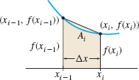
Assume f is nonnegative and continuous on [a,b ]. We seek the area A of the region bounded by the graph of f, the x-axis, and the lines x=a and x=b. We partition the closed interval [a,b] into n subintervals, [a, x_{1}], [x_{1}, x_{2}], \ldots , [x_{i-1}, x_{i}], \ldots , [x_{n-1}, b], each of width \Delta x=\dfrac{b-a}{n}. The y-coordinates corresponding to the numbers x_{0}=a, x_{1}, x_{2}, \ldots , x_{i-1}, x_{i}, \ldots , x_{n}=b are f(x_{0}), f(x_{1}), f(x_{2}), \ldots , f( x_{i-1}) , f(x_{i}) , \ldots, f(x_{n-1}) , f(x_{n}). We connect each pair of consecutive points (x_{i-1}, f( x_{i-1})) and \left( x_{i}, f(x_{i}) \right) , i=1,2, \ldots , n, with a line segment to form n trapezoids. The trapezoid whose base is \Delta x=x_{i}-x_{i-1}=\dfrac{b-a}{n} has parallel sides of lengths f( x_{i-1}) and f(x_{i}) . Based on Figure 12, its area A_{i} is A_{i}=\dfrac{1}{2}\left[f( x_{i-1}) +f(x_{i}) \right] \Delta x
The sum of the areas of the n trapezoids approximates the area A under the graph of f. See Figure 13.
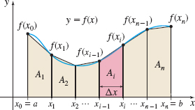
Then \begin{eqnarray*} A &\approx & \dfrac{1}{2}\,[f(x_{0})+f(x_{1})] \,\Delta x+ \dfrac{1}{2}\,[f(x_{1})+f(x_{2})] \,\Delta x+\cdots +\dfrac{ 1}{2}\,[f(x_{n-1}) +f(x_{n})] \,\Delta x \\[6pt] &\approx & \dfrac{1}{2}[f(x_{0})+2f(x_{1})+2f(x_{2})+\cdots +2f(x_{n-1})+f(x_{n})] \Delta x \end{eqnarray*}
Now substitute \Delta x=\dfrac{b-a}{n} to obtain the Trapezoidal Rule.
EXAMPLE 1Approximating \displaystyle\int_{0}^{\pi }\sin x\, dx Using the Trapezoidal Rule
- (a) Use the Trapezoidal Rule with n=4 and n=6 to approximate \int_{0}^{\pi }\sin x\,dx, rounded to three decimal places.
- (b) Compare each approximation to the exact value of \int_{0}^{\pi }\sin xdx.
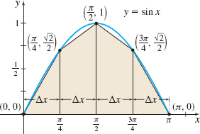
Solution (a) We partition the interval [0,\pi] into four subintervals, each of width \Delta x=\dfrac{\pi -0}{4}=\dfrac{\pi }{4}. \left[ 0,\dfrac{\pi }{4}\right] \qquad \left[ \dfrac{\pi }{4},\dfrac{ \pi }{2}\right]\hbox{} \qquad \left[ \dfrac{\pi }{2},\dfrac{3\pi }{4}\right] \hbox{}\qquad \left[\dfrac{3\pi }{4},\pi \right]
510
The values of f( x) =\sin x corresponding to each endpoint are f(0) =0 \!\qquad f\!\left( \dfrac{\pi }{4} \right) =\dfrac{\sqrt{2}}{2}\!\qquad f\!\left( \dfrac{\pi }{2} \right) =1\!\qquad f\!\left( \dfrac{3\pi }{4}\right) = \dfrac{\sqrt{2}}{2}\!\qquad f (\pi) =0
See Figure 14. Now we use the Trapezoidal Rule: \begin{eqnarray*} \int_{0}^{\pi }\sin x\,dx &\approx &\dfrac{\pi -0}{2\cdot 4}\,\left[ \sin (0)+2\,\sin \left( \dfrac{\pi }{4}\right) +2\,\sin \left( \dfrac{\pi }{2} \right) +2\,\sin \left( \dfrac{3\pi }{4}\right) +\sin (\pi )\right] \\[6pt] &=&\dfrac{\pi }{8}\,\left[ 0+2\left( \dfrac{\sqrt{2}}{2}\right) +2\left( 1\right) +2\left( \dfrac{\sqrt{2}}{2}\right) +0\right] =\dfrac{\pi }{8} \big( 2+2\sqrt{2}\big) \\[6pt] &=& \dfrac{\pi }{4}\big( 1+\sqrt{2}\big) \approx 1.896 \end{eqnarray*}


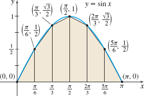
To approximate \int_{0}^{\pi }\sin x\,dx using six subintervals, we partition [0,\pi] into six subintervals, each of width \Delta x=\dfrac{\pi -0}{6}=\dfrac{\pi }{6}, namely, \left[ 0,\dfrac{\pi }{6}\right]\! \qquad \left[ \dfrac{\pi }{6},\dfrac{ \pi }{3}\right]\!\qquad \left[ \dfrac{\pi }{3},\dfrac{\pi }{2}\right]\! \qquad \left[ \dfrac{\pi }{2},\dfrac{2\pi }{3}\right]\!\qquad \left[\dfrac{2\pi }{3},\dfrac{5\pi }{6}\right]\! \qquad \left[ \dfrac{ 5\pi }{6},\pi \right]
See Figure 15. Then we use the Trapezoidal Rule. \begin{eqnarray*} \int_{0}^{\pi }\sin x\,dx &\approx & \dfrac{\pi }{2\cdot 6}\left[ 0+2\cdot \dfrac{1}{2}+2\cdot \dfrac{\sqrt{3}}{2}+2\cdot 1+2\cdot \dfrac{\sqrt{3}}{2} +2\cdot \dfrac{1}{2}+0\right] \\[5pt] &=&\dfrac{\pi }{12}(4+2\sqrt{3}) = \dfrac{\pi }{6}(2+\sqrt{3}) \approx 1.954 \end{eqnarray*}
(b) The exact value of the integral is \int_{0}^{\pi }\sin x \, dx = \big[-\cos x\big] _{0}^{\pi }=-\cos \pi +\cos 0=1+1=2
The approximation using the Trapezoidal Rule with four subintervals underestimates the integral by 0.104. The approximation using six subintervals underestimates the integral by 0.046. Notice that the approximation using six subintervals is more accurate than the approximation using four subintervals.
EXAMPLE 2Approximating \int_{1}^{2}\dfrac{e^{x}}{x}\, dx Using the Trapezoidal Rule
Use the Trapezoidal Rule with n=4 and n=6 to approximate \int_{1}^{2} \dfrac{e^{x}}{x}dx. Express the answer rounded to three decimal places.
Solution We begin by partitioning the interval [1,2] into four subintervals, each of width \Delta x=\dfrac{2-1}{4}=\dfrac{1}{4}: \left[ 1,\,\dfrac{5}{4}\right]\qquad \left[ \dfrac{5}{4},\,\dfrac{3}{2} \right]\qquad \left[ \dfrac{3}{2},\,\dfrac{7}{4}\right]\qquad \left[ \dfrac{7}{4},\,2\right]
The values of f ( x) =\dfrac{e^{x}}{x} corresponding to each endpoint are \begin{eqnarray*} f(1) &=& e \quad f\!\left( \dfrac{5}{4}\right) = \dfrac{4e^{5/4}}{5}\quad f\!\left( \dfrac{3}{2}\right) =\dfrac{2e^{3/2}}{3}\quad f\!\left( \dfrac{7}{4}\right) = \dfrac{4e^{7/4}}{7}\quad f( 2) =\dfrac{e^{2}}{2} \end{eqnarray*}
511
Then, using the Trapezoidal Rule, we get \int_{1}^{2}\dfrac{e^{x}}{x}dx\approx \dfrac{1}{2\cdot 4}\,\left[ e+2\cdot \dfrac{4e^{5/4}}{5}+2\,\cdot \dfrac{2e^{3/2}}{3}+2\,\cdot \dfrac{4e^{7/4}}{7} +\dfrac{e^{2}}{2}\right] \approx 3.069
To approximate \int_{1}^{2}\dfrac{e^{x}}{x}\,dx using six subintervals, we partition [1,2] into six subintervals, each of width \Delta x= \dfrac{2-1}{6}=\dfrac{1}{6}: \left[ 1,\,\dfrac{7}{6}\right]\! \quad \left[ \dfrac{7}{6},\,\dfrac{4}{3} \right]\! \quad \left[ \dfrac{4}{3},\,\dfrac{3}{2}\right]\! \quad \left[ \dfrac{3}{2},\dfrac{5}{3}\right]\!\quad \left[ \dfrac{5}{3},\dfrac{11}{6} \right]\!\quad \left[ \dfrac{11}{6},2\right]
Then, using the Trapezoidal Rule, we get \begin{eqnarray*} \int_{1}^{2}\dfrac{e^{x}}{x}dx\approx \dfrac{1}{2\cdot 6}\,\left[f(1)+2f\! \left( \dfrac{7}{6}\right) +2f\! \left( \dfrac{4}{3}\right) \right.&+& 2f\! \left( \dfrac{3}{2}\right) +2f\! \left( \dfrac{5}{3}\right) \\[5pt] &+& \left. 2f\!\left( \dfrac{11}{6}\right) +f(2) \right] \approx 3.063 \end{eqnarray*}
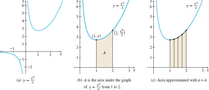
Since f( x) =\dfrac{e^{x}}{x}\gt0 on the interval [1,2 ] , the integral \int_{1}^{2}\dfrac{e^{x}}{x}dx equals the area under the graph of f from 1 to 2. Figure 16 shows the graph of y= \dfrac{e^{x}}{x}, the area A=\int_{1}^{2}\dfrac{e^{x}}{x}dx, and the approximation to the area using the Trapezoidal Rule with four subintervals.
NOW WORK
We cannot find the exact value of the integral \int_{1}^{2}\dfrac{e^{x}}{x} dx. The significance of the Trapezoidal Rule is that not only can it be used to approximate such integrals, but it also provides an estimate of the error, the difference between the exact value of the integral and the approximate value.
512
THEOREM Error in the Trapezoidal Rule
Let f be a function for which f^{\prime \prime} is continuous on some open interval containing a and b. The error in using the Trapezoidal Rule to approximate \int_{a}^{b}f( x) \,dx can be estimated* using the formula \bbox[5px, border:1px solid black, #F9F7ED] {{Error} \leq \dfrac{(b-a)^{3}M}{12n^{2}}}
where M is the absolute maximum value of \vert f^{\prime \prime} \vert on the closed interval [a,b].
*The usefulness of this result is that we can find an upper bound to the error without knowing the exact value of the integral.
NOTE
The error formula gives an upper bound to the error. A derivation of the error formula, which uses an extension of the Mean Value Theorem, may be found in numerical analysis books.
To find M in the error estimate usually involves a lot of computation, so we will use technology to obtain M.
EXAMPLE 3Estimating the Error in Using the Trapezoidal Rule
![]()
Estimate the error that results from using the Trapezoidal Rule with n=4 and with n=6 to approximate \int_{1}^{2}\dfrac{e^{x}}{x}dx. See Example 2.
NOTE
A CAS can be used to find f{^\prime{^\prime}} (x).
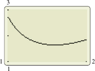
Solution To estimate the error resulting from approximating \int_{1}^{2}\dfrac{e^{x}}{x}dx using the Trapezoidal Rule, we need to find the absolute maximum value of \vert f^{\prime \prime}\vert on the interval [ 1,2] . We begin by finding f^{\prime \prime}: \begin{eqnarray*} f( x) &=&\dfrac{e^{x}}{x} \\[5pt] f^{\prime} (x) &=&\dfrac{d}{dx}\dfrac{e^{x}}{x}=\dfrac{xe^{x}-e^{x}}{x^{2}}= \dfrac{e^{x}}{x}-\dfrac{e^{x}}{x^{2}} \\[5pt] f^{\prime \prime} (x) &=&\dfrac{d}{dx}\left( \dfrac{e^{x}}{x}-\dfrac{e^{x}}{ x^{2}}\right) =\dfrac{d}{dx}\dfrac{e^{x}}{x}-\dfrac{d}{dx}\dfrac{e^{x}}{x^{2} }=\left( \dfrac{e^{x}}{x}-\dfrac{e^{x}}{x^{2}}\right) -\dfrac{ e^{x}x^{2}-2e^{x}x}{x^{4}}\\[5pt] &=&\dfrac{e^{x}}{x}-\dfrac{e^{x}}{x^{2}}-\dfrac{e^{x} }{x^{2}}+\dfrac{2e^{x}}{x^{3}} \\[5pt] &=&e^{x}\left( \dfrac{1}{x}-\dfrac{2}{x^{2}}+\dfrac{2}{x^{3}}\right) \end{eqnarray*}
Since \vert f^{\prime \prime}\vert is continuous on the interval [1,2] , the Extreme Value Theorem guarantees that \vert f^{\prime \prime}\vert has an absolute maximum on [1,2]. We find the absolute maximum of \vert f^{\prime \prime}\vert using graphing technology. As seen from Figure 17, the absolute maximum is at the left endpoint 1. The absolute maximum value of f^{\prime \prime} is \left\vert e^{1}\left( \dfrac{1}{1}-\dfrac{ 2}{1^{2}}+\dfrac{2}{1^{3}}\right) \right\vert =e. So, M=e.
When n=4, the error in using the Trapezoidal Rule is \hbox{Error} \leq \dfrac{( b-a) ^{3}M}{12n^{2}}=\dfrac{(2-1)^{3}(e) }{(12)(4^{2})}=\dfrac{e}{192}\approx 0.014
That is, \begin{eqnarray*} 3.069-0.014 & \leq &\int_{1}^{2}\dfrac{e^{x}}{x}dx \leq 3.069+0.014 \\[5pt] 3.055 & \leq &\int_{1}^{2}\dfrac{e^{x}}{x}dx \leq 3.083 \end{eqnarray*}
513
When n=6, the error in using the Trapezoidal Rule is \hbox{Error} \leq \dfrac{\left( b-a\right) ^{3}M}{12n^{2}}=\dfrac{(2-1)^{3}(e) }{(12)(6^{2})}=\dfrac{e}{432}\approx 0.006
That is, \begin{eqnarray*} 3.063-0.006 & \leq &\int_{1}^{2}\dfrac{e^{x}}{x}dx \leq 3.063+0.006 \nonumber \\[5pt] 3.057 & \leq &\int_{1}^{2}\dfrac{e^{x}}{x}dx \leq 3.069 \end{eqnarray*}
NOW WORK
EXAMPLE 4Obtaining a Desired Accuracy Using the Trapezoidal Rule
Find the number of subintervals n needed to guarantee that the Trapezoidal Rule approximates \int_{1}^{2}\dfrac{e^{x}}{x}dx correct to within 0.0001.
Solution To be sure that the approximation of \int_{1}^{2} \dfrac{e^{x}}{x}dx is correct to within 0.0001, we require the error be less than 0.0001. That is, \begin{eqnarray*} \hbox{Error} & \leq & \dfrac{(b-a)^{3}M}{12n^{2}}=\dfrac{(2-1)^{3}M}{12n^{2}}\underset{\underset{\color{#0066A7}{M=e}}{\color{#0066A7}{\uparrow}}} {=}\dfrac{e}{12n^{2}} \lt 0.0001 \\ n^{2} & \gt &\dfrac{e}{(0.0001) (12) }=\dfrac{e}{0.0012} \\ n & \gt &{\sqrt{\dfrac{e}{0.0012}}}\approx 47.6 \end{eqnarray*}
To ensure that the error is less than 0.0001, we round up to 48 subintervals.
NOW WORK
The Trapezoidal Rule is very useful in applications when only experimental (empirical) data are available.

EXAMPLE 5Using the Trapezoidal Rule with Empirical Data
A 140-foot ({\rm ft}) tree trunk is cut into 20-ft logs. The diameter of each cross-sectional cut is measured and its area A recorded in the table below. (x is the distance in feet of the cut from the top of the trunk.)
| x({\rm ft}) | 0 | 20 | 40 | 60 | 80 | 100 | 120 | 140 |
| A({\rm ft^{2}}) | 120 | 124 | 128 | 130 | 132 | 136 | 144 | 158 |
Find the approximate volume of the tree trunk.
Solution The volume of the tree trunk is V=\int_{0}^{140}A ( x) \,dx, where A( x) is the area of a slice at x. Since only eight data points are given, the function A( x) is not explicitly known. To approximate the volume, we partition the interval [ 0,140] into seven subintervals, each of width \Delta x=\dfrac{140}{7}=20. This partition corresponds to the given data. Using the Trapezoidal Rule, the approximate volume of the tree trunk is \begin{eqnarray*} V= \int_{0}^{140}A( x) \,dx\approx \dfrac{1}{2}(20) \,[ A(0)+2\,A\,(20)&+&2\,A(40)+2\,A (60) +2\,A(80) \\[5pt] &+& 2\,A (100) +2\,A(120) +A\,(140)] \end{eqnarray*} \begin{eqnarray*} V &\approx & 10\,[120+2(124)+2(128)+2(130)+2(132)+2(136)+2(144)+158]\\[5pt] &=& 18{,}660 \end{eqnarray*}
514
The volume of the tree trunk is approximately 18{,}660{\rm ft^{3}}.
NOW WORK
2 Approximate an Integral Using Simpson’s RulePrinted Page 514
NOTE
With the Trapezoidal Rule, we approximate a function f with line segments (first degree polynomials), whereas with Simpson’s Rule, we approximate f with parabolic arcs (second degree polynomials).
Another way to approximate the definite integral of a function f that is continuous on a closed interval [a,b], is called Simpson’s Rule. Simpson’s Rule, which approximates \int_{a}^{b} f( x) \,dx using parabolic arcs, instead of line segments as in the Trapezoidal Rule, often gives a better approximation to the area A.
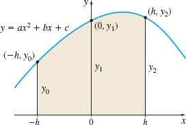
Before stating Simpson’s Rule, we derive a formula for the area A under a parabolic arc. Let the graph in Figure 18 represent the parabola y=ax^{2}+bx+c. Draw the lines x=-h and x=h, so that the points (-h, y_{0}), (0, y_{1}), and (h, y_{2}) lie on the parabola.
The area A enclosed by the parabola, the x-axis, and the lines x=-h and x=h is given by \begin{eqnarray*} A&=& \int_{-h}^{h}y\,dx=\int_{-h}^{h}(ax^{2}+bx+c)\,dx=\left[ a\dfrac{ x^{3}}{3}+b\dfrac{x^{2}}{2}+cx \right] _{-h}^{h} \nonumber\\[5pt] &=&\dfrac{2}{3}ah^{3}+2ch= \dfrac{h}{3}(2ah^{2}+6c)\tag{1} \end{eqnarray*}
Since the parabola contains the points (-h,\,y_{0}), ( 0,\,y_{1}), and (h,\,y_{2}), each point must satisfy the equation y=ax^{2}+bx+c, and we have the system of equations: \begin{eqnarray*} \begin{array}{rl@{\qquad}rl} y_{0}&=ah^{2}-bh+c &\qquad {\hbox{\({\color{#0066A7}x} {\color{#0066A7}=} {\color{#0066A7}-}{\color{#0066A7}h}\)}} \\ y_{1}&=c &\qquad {\hbox{\({\color{#0066A7}x} {\color{#0066A7}=} {\color{#0066A7}0}\)}} \\ y_{2}&=ah^{2}+bh+c &\qquad {\hbox{\({\color{#0066A7}x} {\color{#0066A7}=} {\color{#0066A7}h}\)}} \end{array} \end{eqnarray*}
Adding the first and third equations gives y_{0}+y_{2}=2ah^{2}+2c
Add 4y_{1}=4c to each side. y_{0}+y_{2}+4y_{1}=2ah^{2}+6c
Then substitute y_{0}+y_{2}+4y_{1} for 2ah^{2}+6c in formula (1) for the area A to obtain \begin{equation*} A=\dfrac{h}{3}(y_{0}+4y_{1}+y_{2})\tag{2} \end{equation*}
This formula for A depends on only y_{0}, y_{1}, y_{2}, and the distance h.
Now assume that a function f is nonnegative and continuous on [a,b ]. Then the area A under the graph of f, A=\int_{a}^{b} f ( x) \,dx, can be approximated by partitioning the interval [a,b ] into an even number n of subintervals, each of width \Delta x=\dfrac{b-a}{n}. The y-coordinates corresponding to the numbers x_{0}=a, x_{1}, x_{2}, \ldots , x_{i-1}, x_{i}, \ldots , x_{n}=b are f(x_{0}), f(x_{1}), f(x_{2}), \ldots , f( x_{i-1}) , f(x_{i}) , \ldots , f(x_{n-1}), f(x_{n}). We connect each triple of points ( x_{i-1}, f( x_{i-1})) (x_{i}, f(x_{i})), and ( x_{i+1}, f(x_{i+1})), i=1,3,5,\ldots , n-1 with parabolic arcs, and use (2) to find the area A_{i} enclosed by the arc centered at ( x_{i},f(x_{i}) ) and the lines x=x_{i-1} and x=x_{i+1}. With h=\Delta x=\dfrac{b-a}{n}, we have A_{i}=\dfrac{b-a}{3n}[f (x_{i-1}) +4f(x_{i}) +f (x_{i+1} )]
515
The sum of these areas gives an approximation to A=\int_{a}^{b}f( x)\,dx.
ORIGINS
Simpson’s Rule is named after the British mathematician Thomas Simpson, who lived from 1710 to 1761.
Simpson’s Rule
If a function f is continuous on the closed interval [a,\,b], then \bbox[5px, border:1px solid black, #F9F7ED]{ \begin{array}{lll} \int_{a}^{b}f(x)\,dx \approx \dfrac{b-a}{3n} [ f(x_{0})&+&4 f(x_{1})+2 f(x_{2})+4 f(x_{3})+2f(x_{4}) \\[8pt] && + \cdots + 2f(x_{n-2})+4 f(x_{n-1})+f(x_{n})] \end{array} }
where the closed interval [a,b] is partitioned into an even number n of subintervals [x_{0}, x_{1}], [x_{1}, x_{2}], \ldots , [x_{n-1}, x_{n}], each of width \dfrac{b-a}{n}.
A proof of Simpson’s Rule that does not assume f is nonnegative can be found in most numerical analysis books.
EXAMPLE 6Approximating an Integral Using Simpson’s Rule
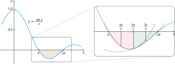
Use Simpson’s Rule with n=4 to approximate \int_{\pi }^{2\pi }\dfrac{\sin x}{x}dx. Express the answer rounded to three decimal places.
Solution We partition the interval [\pi ,2\pi ] into the four subintervals \left[ \pi ,\dfrac{5\pi }{4}\right]\!\qquad \left[ \dfrac{5\pi }{4},\dfrac{ 3\pi }{2}\right]\!\qquad \left[ \dfrac{3\pi }{2},\dfrac{7\pi }{4}\right]\!\qquad \left[ \dfrac{7\pi }{4},2\pi \right]
each of width \dfrac{\pi }{4}. The value of f( x) =\dfrac{\sin x}{x} corresponding to each endpoint is \begin{eqnarray*} f(\pi) &=& 0\ \ \ f\!\left( \dfrac{5\pi }{4}\right) = - \dfrac{2\sqrt{2}}{5\pi}\ \ \ f\!\left( \dfrac{3\pi }{2} \right) =-\dfrac{2}{3\pi}\ \ \ f\!\left( \dfrac{7\pi }{4}\right) = -\dfrac{2\sqrt{2}}{7\pi}\quad f(2\pi) =0 \end{eqnarray*}
Then using Simpson’s Rule, we get \begin{eqnarray*} \int_{\pi }^{2\pi }\dfrac{\sin x}{x}\,dx &\approx &\dfrac{2\pi -\pi }{3\cdot 4} \left[ f(\pi )+4\, f\! \left( \dfrac{5\pi }{4}\right) +2 f\! \left( \dfrac{3\pi }{2}\right) +4 f\! \left( \dfrac{7\pi }{4}\right) +f( 2\pi ) \right] \nonumber \\[7pt] &= &\left( \dfrac{\pi }{12}\right) \left[ 0+4\left( -\dfrac{2\sqrt{2}}{ 5\pi }\right) +2\left( -\dfrac{2}{3\pi }\right) +4\left( -\dfrac{2\sqrt{2}}{ 7\pi }\right) +0\right] \approx -0.434 \end{eqnarray*}
The graph of y=\dfrac{\sin x}{x} is shown in Figure 19 on page 516.
516
THEOREM Error in Simpson’s Rule
Let f be a function for which f^{(4)} is continuous on an open interval containing a and b. The error in using Simpson’s Rule to approximate \int_{a}^{b}f(x)\,dx can be estimated by the formula \bbox[5px, border:1px solid black, #F9F7ED]{ \hbox{Error} \leq \frac{(b-a)^{5}M}{180n^{4}}}
where M is the absolute maximum value of \vert f^{\,(4)}(x)\vert on the closed interval [a,b].
As with the Trapezoidal Rule, the error formula gives an upper bound to the error. A derivation of the error formula, which uses an extension of the Mean Value Theorem, may be found in numerical analysis books.
To find M in the error estimate usually involves a lot of computation. So, we use technology to find M.
NOTE
A CAS can be used to find higher-order derivatives.
EXAMPLE 7Estimating the Error in Using Simpson's Rule
![]()
Estimate the error that results from using Simpson's Rule with n =4 to approximate \int_{\pi }^{2\pi }\frac{\sin x}{x}dx. (See Example 6.)
Solution To estimate the error, we need to find the absolute maximum value of \vert f^{(4) }\vert on the interval [\pi ,2\pi ]. We begin by finding f^{(4) }: \begin{eqnarray*} f(x) &=&\dfrac{\sin x}{x} \\[5pt] f^{\prime} (x) &=&\frac{x\cos x-\sin x}{x^{2}}=\frac{\cos x}{x}-\frac{\sin x}{x^{2}} \\ && \\ f^{\prime \prime} (x) &=&\left[ \frac{-x\sin x-\cos x}{x^{2}} \right] -\left[ \frac{x^{2}\cos x-2x\sin x}{x^{4}}\right]\\[6pt] & = & \frac{2 \sin x}{x^{3}} -\frac{\sin x}{x}-\frac{2\cos x}{x^{2}} \\[15pt] f^{\prime \prime \prime} (x) &=&\left[ \frac{2x^{3}\cos x-6x^{2}\sin x}{x^{6}}\right] -\left[ \frac{x\cos x-\sin x}{x^{2}}\right] - \left[ \frac{-2x^{2}\sin x-4x\cos x}{x^{4}}\right] \\[6pt] &=&\frac{2\cos x}{x^{3}}-\frac{6\sin x}{x^{4}}-\frac{\cos x}{x}+\frac{ \sin x}{x^{2}}+\frac{2\sin x}{x^{2}}+\frac{4\cos x}{x^{3}}\\[6pt] &=&\frac{6 \cos x}{x^{3}}-\frac{\cos x}{x}+\frac{3 \sin x}{x^{4}} \\[6pt] && \\ f^{\,(4) }(x) &=&\left[ \frac{-6x^{3}\sin x-18x^{2}\cos x}{ x^{6}}\right] -\left[ \frac{-x\sin x-\cos x}{x^{2}}\right] \\[8pt] &&+\,\left[ \frac{3x^{2}\cos x-6x\sin x}{x^{4}}\right] -\left[ \frac{6x^{4}\cos x-24x^{3}\sin x}{x^{8}}\right] \\[8pt] &=&\frac{4 \cos x}{x^{2}}-\frac{24 \cos x}{x^{4}}+\frac{\sin x}{x}-\frac{ 12 \sin x}{x^{3}}+\frac{24 \sin x}{x^{5}} \end{eqnarray*}
517
We use graphing technology to find the absolute maximum value of \vert f^{(4)}\vert. See Figure 20.
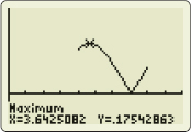
Since on the interval [\pi ,2\pi] the maximum value of \vert f^{(4)}\vert \lt 0.176, we use M=0.176. Then the error that results from using Simpson's Rule to approximate \int_{\pi }^{2\pi }\frac{\sin x}{x}dx is \hbox{Error} \leq \frac{M(b-a)^{5}}{180n^{4}}=\frac{0.176(2\pi -\pi )^{5}}{180\cdot 4^{4}}\approx 0.001
That is, \begin{eqnarray*} -0.434-0.001 & \leq& \int_{\pi }^{2\pi }\frac{\sin x}{x}dx \leq -0.434+0.001 \\[5pt] -0.435 & \leq& \int_{\pi }^{2\pi }\frac{\sin x}{x}dx \leq -0.433 \end{eqnarray*}
NOW WORK
EXAMPLE 8Obtaining a Desired Accuracy Using Simpson’s Rule
Find the number of subintervals needed to guarantee that Simpson’s Rule approximates \int_{\pi }^{2\pi }\frac{\sin x}{x}\, dx correct to within 0.0001.
Solution To be sure that the approximation of \int_{\pi }^{2\pi } \frac{\sin x}{x}dx is correct to within 0.0001, we require the error be less than 0.0001. That is, \begin{eqnarray*} \hbox{Error} & \leq &\dfrac{(b-a)^{5}M}{180n^{4}}=\dfrac{(2\pi -\pi )^{5}M}{180n^{4}} &&\underset{\underset{\color{#0066A7}{M=0.176}}{\color{#0066A7}{{\uparrow }}}}{=} \dfrac{( \pi ^{5}) (0.176) }{180n^{4}} \lt 0.0001 \\[-8pt] n^{4} &>&\dfrac{0.176\pi ^{5}}{(0.0001) \left( 180\right) } \\[6pt] n &>&\sqrt[4]{2992.192}\approx 7.396 \end{eqnarray*}
Since Simpson's Rule requires n to be even, eight subintervals are needed to guarantee that Simpson's Rule approximates \int_{\pi }^{2\pi }\frac{\sin x }{x} dx correct to within 0.0001.