15.7 Surface and Flux IntegralsPrinted Page 1027
1027
Surface integrals are similar to line integrals, but the integration takes place on a surface instead of along a curve.
Suppose the smooth surface S has the parametrization r(u,v)=x(u,v)i+y(u,v)j+z(u,v)k
and its parameter domain R is a closed, bounded region of the uv-plane. Then following our usual practice, we partition a rectangular region containing R into subrectangles using lines parallel to the u-axis and the v-axis and discard any subrectangles not lying entirely in R. Suppose we are left with n subrectangles Rk, k=1,2,…,n, with width Δuk and height Δvk. The area of the subrectangle Rk is ΔAk=ΔukΔvk.
The kth subrectangle Rk is formed by the lines u=uk, u=uk+Δuk, v=vk, and v=vk+Δvk. The portions of the lines forming the edges of the subrectangle Rk map to portions of their corresponding coordinate curves on the surface S. That is, each subrectangle Rk maps into a closed curved patch Sk on S whose area is ΔSk. We define the norm ‖ to be the largest area \Delta S_{k}. We now choose a point P_{k}=(u_{k}^{\ast },v_{k}^{\ast }) in each subrectangle.
Let w=F(x,y,z) be a function that is defined over a solid in space containing the surface S. We evalute F at the point (x(u^*_k,v^*_k), y(u^*_k,v^*_k), z(u^*_k,v^*_k) ) on S_{k} and form the product F(x(u^*_k,v^*_k), y(u^*_k,v^*_k), z(u^*_k,v^*_k) )\Delta S_{k}. Now we add obtaining the sums \sum_{k=1}^{n}F(x(u^*_k,v^*_k), y(u^*_k,v^*_k), z(u^*_k,v^*_k))\,\Delta S_{k}
Then we have the following definition.
DEFINITION Surface Integral
Let S be a surface defined on a closed, bounded region R with a smooth parametrization \mathbf{r}(u,v) =x(u,v) \mathbf{i}+y(u,v) \mathbf{j} +z(u,v) \mathbf{k}. Also, let w= F(x,y,z) be defined over a solid containing the surface S. Then the surface integral of F over S is defined as \bbox[5px, border:1px solid black, #F9F7ED]{\bbox[#FAF8ED,5pt]{ \iint\limits_{\kern-3ptS}F(x,y,z)\,dS=\lim\limits_{\Vert \Delta \Vert \rightarrow 0}\sum\limits_{k=1}^{n} F\left(x\left( u_{k}^{\ast },v_{k}^{\ast }\right)\, y\left(u_{k}^{\ast },v_{k}^{\ast }\right)\,z\left( u_{k}^{\ast },v_{k}^{\ast }\right) \right) \Delta S_{k} }}
provided this limit exists.
1 Find a Surface Integral Using a Double IntegralPrinted Page 1027
When the function w=F( x,y,z) is continuous on some solid that contains S, the surface integral of F over S can be expressed as a double integral.
THEOREM A Surface Integral Expressed as a Double Integral
Let S be a surface defined on a closed, bounded region R with a smooth parametrization \mathbf{r}(u,v) =x(u,v) \mathbf{i}+y(u,v) \mathbf{j} +z(u,v) \mathbf{k}. Also, suppose that w=F(x,y,z) is continuous on a solid containing the surface S. Then the surface integral of F over S is given by \begin{equation*} \bbox[5px, border:1px solid black, #F9F7ED]{\bbox[#FAF8ED,5pt]{\iint\limits_{\kern-3ptS}F(x,y,z)\,dS=\iint\limits_{\kern-3ptR}F(x(u,v) ,y(u,v) ,\,z(u,v))\left\Vert \mathbf{r} _{u}\times \mathbf{r}_{v}\right\Vert \,du\,dv } } \tag{1} \end{equation*}
1028
It is important to note that just as a line integral does not depend on the parame- trization used, surface integrals do not depend on the smooth parametrization used in the integration. Also, there are occasions when we want to find a surface integral over a piecewise-smooth surface. A piecewise-smooth surface is a finite collection of smooth surfaces that intersect only along piecewise-smooth curves. In these cases, just as with line integrals, we integrate over each smooth surface separately and then sum the results.
EXAMPLE 1Finding a Surface Integral
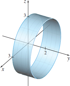
Find \iint\limits_{\kern-3ptS}ye^{x^{2}+z^{2}}dS, where S is the part of the surface of the cylinder x^{2}+z^{2}=9 that lies between y=0 and y=2.
Solution The surface S is shown in Figure 52. Since the surface is a piece of a cylinder, we use a variation of cylindrical coordinates to parametrize the surface. Here, we use x=r\cos \theta , y=y, and z=r\sin \theta . (Do you see why?) Then r^{2}=x^{2}+z^{2}=9, so r=3. We parametrize the surface S using \begin{equation*} \mathbf{r}( \theta ,y) =3\cos \theta\ \mathbf{i}+y\mathbf{j}+3\sin \theta\ \mathbf{k} \end{equation*}
where the parameter domain {R} is 0\leq \theta \leq 2\pi and 0\leq y\leq 2.
The partial derivatives of \mathbf{r} are \mathbf{r}_{\theta }( \theta ,y) =-3\sin \theta\ \mathbf{i}+3\cos \theta\ \mathbf{k}\qquad\hbox{and}\qquad \mathbf{r}_{y}( \theta ,y) =\mathbf{j}
and their cross product is \begin{equation*} \mathbf{r}_{\theta }\times \mathbf{r}_{y}= \left|\begin{array}{c@{\quad}c@{\quad}c} \mathbf{i} & \mathbf{j} & \mathbf{k} \\ -3\sin \theta & 0 & 3\cos \theta \\ 0 & 1 & 0 \end{array}\right| =-3\cos \theta\ \mathbf{i}-3\sin \theta\ \mathbf{k} \end{equation*}
Then \left\Vert \mathbf{r}_{\theta }\times \mathbf{r}_{y}\right\Vert =\sqrt{9\cos ^{2}\theta +9\sin ^{2}\theta }=3. So, we have \begin{eqnarray*} \iint\limits_{\kern-3ptS}ye^{x^{2}+z^{2}}dS &=&\iint\limits_{\kern-3ptR}ye^{9}\left\Vert \mathbf{r}_{\theta }\times \mathbf{r}_{y}\right\Vert d\theta dy=\int_{0}^{2}\int_{0}^{2\pi }( ye^{9}) 3\,d\theta\, dy \notag \\[4pt] &=&3e^{9}\int_{0}^{2}y\big[ \theta \big] _{0}^{2\pi }dy=3e^{9}\int_{0}^{2}2\pi y\,dy=6\pi e^{9}\left[ \dfrac{y^{2}}{2}\right] _{0}^{2}=12\pi e^{9} \end{eqnarray*}
RECALL
A lamina is a thin, flat sheet of material.
NOW WORK
The formulas for finding the center of mass of a lamina can be generalized. The following formulas for the center of mass of a general lamina with variable mass density \rho =\rho ( x,y,z) in the shape of a surface S result from a derivation similar to that found in Section 14.4 for a flat sheet.
NEED TO REVIEW?
The center of mass of a lamina with variable density is discussed in Section 14.4, pp. 929-932.
\bbox[5px, border:1px solid black, #F9F7ED]{\bbox[#FAF8ED,5pt]{ \begin{array}{r@{\qquad}rcl} \hbox{Mass of \(S\):} & M&=&\iint\limits_{\kern-3ptS}\rho ( x,y,z) \,dS \\ \hbox{Moment about the \(yz\)-plane:} & M_{yz}&=&\iint\limits_{\kern-3ptS}x\rho ( x,y,z) \,dS\\ \hbox{Moment about the \(xz\)-plane:} & M_{xz}&=&\iint\limits_{\kern-3ptS}y\rho ( x,y,z) \,dS\\ \hbox{Moment about the \(xy\)-plane:} & M_{xy}&=&\iint\limits_{\kern-3ptS}z\rho ( x,y,z) \,dS\\ \hbox{Center of mass:} & ( \overline{x},\overline{y},\overline{z}) &=&\left( \dfrac{M_{yz}}{M},\dfrac{M_{xz}}{M},\dfrac{M_{xy}}{M}\right) \end{array} }}
1029
EXAMPLE 2Finding the Mass of a Lamina
A lamina in the shape of the cone z=6-\sqrt{x^{2}+y^{2}} lies between the planes z=2 and z=5. If the mass density of the lamina is \rho (x,y,z)=\sqrt{x^{2}+y^{2}}, find the mass M of the lamina.
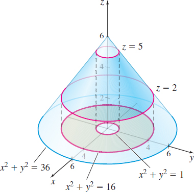
Solution Figure 53 illustrates the lamina. Using x=r\cos \theta , y=r\sin \theta , and z=6-\sqrt{x^{2}+y^{2}}=6-r, we parametrize the surface as \mathbf{r}=\mathbf{r}\left( r,\theta \right) =r\cos \theta \,\mathbf{i} +r\sin \theta \,\mathbf{j}+\left( 6-r\right) \mathbf{k}\qquad 0\leq \theta \leq 2\pi\quad 1\leq r\leq 4
First we find \mathbf{r}_{r}\times \mathbf{r}_{\theta }. \begin{eqnarray*} \mathbf{r}_{r}\times \mathbf{r}_{\theta } &=& \left|\begin{array}{c@{\quad}c@{\quad}c} \mathbf{i} & \mathbf{j} & \mathbf{k} \\ \cos \theta & \sin \theta & -1 \\ -r\sin \theta & r\cos \theta & 0 \end{array}\right| =r\cos \theta \,\mathbf{i} + r\sin \theta \,\mathbf{j}+\left( r\cos ^{2}\theta +r\sin ^{2}\theta \right) \mathbf{k}\\ &=&r\cos \theta \,\mathbf{i}+r\sin \theta \,\mathbf{j}+r\,\mathbf{k} \\[4pt] \hspace{-2pt}\left\Vert \mathbf{r}_{r}\times \mathbf{r}_{\theta }\right\Vert &=&\sqrt{r^{2}\cos ^{2}\theta +r^{2}\sin ^{2}\theta +r^{2}}=r\sqrt{\cos ^{2}\theta +\sin ^{2}\theta +1}=r\sqrt{1+1}=\sqrt{2}\,r \end{eqnarray*}
Since the mass density of the lamina is \rho (x,y,z)=\sqrt{x^{2}+y^{2}}=r and dS=\left\Vert \mathbf{r}_{r}\times \mathbf{r}_{\theta }\right\Vert dr\,d\theta =\sqrt{2}r\,dr\,d\theta , the mass M of the lamina is given by \begin{eqnarray*} M &=&\iint\limits_{\kern-3ptS}\rho (x,y,z)\,dS=\iint\limits_{\kern-3ptR}\rho \left\Vert \mathbf{r}_{r}\times \mathbf{r}_{\theta }\right\Vert dr\,d\theta =\iint\limits_{\kern-3ptR}r(\sqrt{2}r) dr\,d\theta \\ &=&\sqrt{2}\int_{0}^{2\pi }\int_{1}^{4}r^{2}\,dr\,d\theta =\sqrt{2} \int_{0}^{2\pi }\left[ \dfrac{r^{3}}{3}\right] _{1}^{4}\,d\theta =21\sqrt{2} \int_{0}^{2\pi }d\theta =42\sqrt{2}\,\pi \end{eqnarray*}
NOW WORK
RECALL
The centroid is the geometric center of a lamina, and it is numerically equivalent to the center of mass of a homogeneous lamina that has mass density \rho =1.
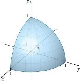
EXAMPLE 3Finding the Centroid of a Surface
Find the centroid of the part of the unit sphere that lies in the first octant. See Figure 54.
Solution In spherical coordinates, the equation of the unit sphere S: x^{2}+y^{2}+z^{2}=1 is \rho =1. So using x=\cos \theta \sin \phi , y=\sin \theta \sin \phi , and z=\cos \phi, we obtain the parametrization \mathbf{r}=\mathbf{r}\left( \theta ,\phi \right) =\cos \theta \sin \phi \, \mathbf{i}+\sin \theta \sin \phi \,\mathbf{j}+\cos \phi\, \mathbf{k};\qquad 0\leq \theta \leq \dfrac{\pi }{2},\quad 0\leq \phi \leq \dfrac{\pi }{2}
We seek \left\Vert \mathbf{r}_{\theta }\times \mathbf{r}_{\phi }\right\Vert and dS. The partial derivatives of \mathbf{r}=\mathbf{r}\left( \theta ,\phi \right) are \begin{eqnarray*} \mathbf{r}_{\theta }&=&-\sin \theta \sin \phi \,\mathbf{i}+\cos \theta \sin \phi \,\mathbf{j} \,\quad \mathbf{r}_{\phi }=\cos \theta \cos \phi \,\mathbf{i}+\sin \theta \cos \phi \,\mathbf{j}-\sin \phi\, \mathbf{k}\\[4pt] \mathbf{r}_{\theta }\times \mathbf{r}_{\phi } &=&\left|\begin{array}{c@{\quad}c@{\quad}c} \mathbf{i} & \mathbf{j} & \mathbf{k} \\[3pt] -\sin \theta \sin \phi & \cos \theta \sin \phi & 0 \\[3pt] \cos \theta \cos \phi & \sin \theta \cos \phi & -\sin \phi \end{array}\right|\\[4pt] &=&-\cos \theta \sin ^{2}\phi \,\mathbf{i}-\sin \theta \sin ^{2}\phi \,\mathbf{ j}-\sin \phi \cos \phi\, \mathbf{k} \\[4pt] \left\Vert \mathbf{r}_{\theta }\times \mathbf{r}_{\phi }\right\Vert &=&\sqrt{ \cos ^{2}\theta \sin ^{4}\phi +\sin ^{2}\theta \sin ^{4}\phi +\sin ^{2}\phi \cos ^{2}\phi }\\[4pt] &=&\sqrt{( \cos ^{2}\theta +\sin ^{2}\theta ) \sin ^{4}\phi +\sin ^{2}\phi \cos ^{2}\phi } \\[4pt] &=&\sqrt{\sin ^{2}\phi (\sin ^{2}\phi +\cos ^{2}\phi) }=\sin \phi\\[4pt] dS&=&\left\Vert \mathbf{r}_{\theta }\times \mathbf{r}_{\phi }\right\Vert d\theta\, d\phi =\sin \phi \,d\theta \,d\phi \end{eqnarray*}
1030
Since the surface area S of a sphere is S=4\pi r^{2}, the surface area of the part of the unit sphere r=1 in the first octant is \dfrac{1}{8}S=\dfrac{\pi }{2}, so the mass M is \dfrac{\pi }{2}. Because of symmetry, \overline{x}=\overline{y}=\overline{z}, so we need to find only one moment, say M_{xy}. \begin{eqnarray*} M_{xy}&=&\iint\limits_{\kern-3ptS}z\,dS=\iint\limits_{\kern-3ptS}\cos \phi \,dS=\int_{0}^{\pi /2}\int_{0}^{\pi /2}\cos \phi\, \sin \phi\, d\theta\, d\phi\\[4pt] &=&\int_{0}^{\pi /2}\dfrac{\pi }{2}\cos \phi\, \sin \phi\, d\phi =\dfrac{\pi }{2}\left[ \dfrac{\sin ^{2}\phi }{2}\right] _{0}^{\pi /2}=\dfrac{\pi }{4} \end{eqnarray*}
The centroid of the part of the unit sphere in the first octant is \left( \overline{x},\overline{y},\overline{z}\right) =\left( \dfrac{M_{yz}}{M },\dfrac{M_{xz}}{M},\dfrac{M_{xy}}{M}\right) =\left( \dfrac{1}{2},\dfrac{1}{2},\dfrac{1}{2} \right)
2 Determine the Orientation of a SurfacePrinted Page 1030
NEED TO REVIEW?
Unit normal vectors are discussed in Section 11.2, pp. 769-770.
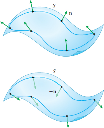
Suppose the surface S has a tangent plane at each point, except possibly at its boundary points. Then there are two unit normal vectors, \mathbf{n}_{1} and \mathbf{n}_{2}\mathbf{,} where \mathbf{n}_{1}=-\mathbf{n}_{2}, that can be drawn at each point of S. See Figure 55.
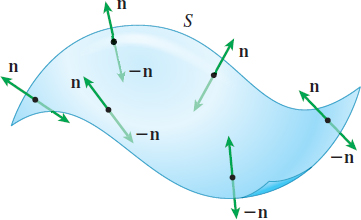
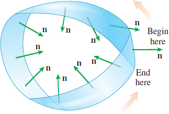
Suppose it is possible to choose a unit normal vector \mathbf{n} at each point of the surface S so that \mathbf{n} varies continuously over the surface, and as \mathbf{n} moves around any closed curve on S, \mathbf{ n} returns to its original direction, as shown in Figure 56. Such a surface is said to be orientable, with the vector \mathbf{n} providing its orientation. As a result, a surface S that is orientable has two possible orientations, one for \mathbf{n} and one for -\mathbf{n}.
Suppose S has a smooth parametrization \mathbf{r}=\mathbf{r}(u,v) , and (u_{0},v_{0}) is in the parameter domain R. Then the vector \mathbf{r}_{u}(u_{0},v_{0}) \times \mathbf{r} _{v}(u_{0},v_{0}) is normal to the tangent plane at \mathbf{r}(u_{0},v_{0}) , and the two unit vectors normal to the surface S are \begin{equation*} \mathbf{n}=\dfrac{\mathbf{r}_{u}\times \mathbf{r}_{v}}{\left\Vert \mathbf{r} _{u}\times \mathbf{r}_{v}\right\Vert }\qquad\hbox{and}\qquad -\mathbf{n}=-\dfrac{ \mathbf{r}_{u}\times \mathbf{r}_{v}}{\left\Vert \mathbf{r}_{u}\times \mathbf{ r}_{v}\right\Vert } \tag{2} \end{equation*}
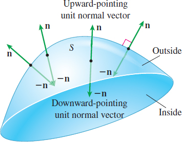
When S is defined by the graph of a function z=f(x,y) , then the two orientations can be called upward and downward depending on the sign of the vector component \mathbf{k}. For general surfaces, there is no natural choice for up and down.
Suppose F( x,y,z) =z-f(x,y) . Then the two unit vectors normal to S are \bbox[5px, border:1px solid black, #F9F7ED]{\bbox[#FAF8ED,5pt]{ \mathbf{n}=\dfrac{{\mathbf\nabla }F}{\Vert {\mathbf\nabla } F\Vert }=\dfrac{-f_{x}(x,y)\mathbf{i}-f_{y}(x,y)\mathbf{j}+\mathbf{k}}{\sqrt{ [f_{x}(x,y)]^{2}+[f_{y}(x,y)]^{2}+1}} } } \tag{3}
and \bbox[5px, border:1px solid black, #F9F7ED]{\bbox[#FAF8ED,5pt]{ -\mathbf{n}=\dfrac{-{\mathbf\nabla }F}{\Vert {\mathbf\nabla }F\Vert }=\dfrac{f_{x}(x,y)\mathbf{i}+f_{y}(x,y)\mathbf{j}-\mathbf{k} }{\sqrt{[f_{x}(x,y)]^{2}+[f_{y}(x,y)]^{2}+1}} }} \tag{4}
NOTE
When F( x,y,z) =z-f(x,y), then S is the level surface F( x,y,z) =0. Level surfaces are discussed in Section 12.1, pp. 812-815.
Since the \mathbf{k} component of \mathbf{n} is positive, it points in the upward direction. For this reason, \mathbf{n} is called the upward-pointing unit normal vector of S. The \mathbf{k} component of -\mathbf{n} is negative. So, -\mathbf{n} is called the downward-pointing unit normal vector of S. Using the two unit vectors, we define the positive side or outside of S as the side associated with the upward-pointing unit vector, and the negative side or inside of S as the side associated with the downward-pointing unit vector. See Figure 57.
1031
EXAMPLE 4Finding the Orientations of a Surface
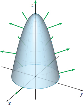
Find both orientations for the paraboloid defined by z=9-x^{2}-y^{2}, z\geq 0.
- (a) Use rectangular coordinates to find the unit normal vectors.
- (b) Parametrize the surface, and then find the unit normal vectors.
Solution (a) Since the paraboloid is given by f(x,y) = 9-x^{2} - y^{2}, z \ge 0, we can use the equations (3) and (4) to find the unit normal vectors. We begin by finding the partial derivatives f_{x}(x,y) =-2x \qquad f_{y}(x,y) =-2y
Then \begin{eqnarray*} \mathbf{n}&=&\dfrac{2x\,\mathbf{i}+2y\,\mathbf{j}+\mathbf{k}}{\sqrt{[-2x]^{2}+[-2y]^{2}+1}}=\dfrac{2x\,\mathbf{i}+2y\,\mathbf{j}+\mathbf{k}}{\sqrt{4x^{2}+4y^{2}+1}} \\[7pt] -\mathbf{n}&=&\dfrac{-2x\,\mathbf{i-}2y\,\mathbf{j}-\mathbf{k}}{\sqrt{[-2x]^{2}+[-2y]^{2}+1}}=\dfrac{ -2x\,\mathbf{i}-2y\,\mathbf{j}-\mathbf{k}}{\sqrt{4x^{2}+4y^{2}+1}} \end{eqnarray*}
Notice that the \mathbf{k} component of \mathbf{n} is positive, indicating \mathbf{n} is the upward-pointing unit normal vector.
(b) We parametrize z=9-x^{2}-y^{2}, z\geq 0, using cylindrical coordinates, by defining the parametric equations \begin{equation*} x=r\cos \theta \qquad y=r\sin \theta \qquad z=9-(x^{2}+y^{2}) =9-r^{2} \end{equation*}
Then the parametrization is \begin{equation*} \mathbf{r}=\mathbf{r}( r,\theta ) =r\cos \theta \,\mathbf{i} +r\sin \theta \,\mathbf{j}+( 9-r^{2}) \mathbf{k} \end{equation*}
We seek \left\Vert \mathbf{r}_{r}\times \mathbf{r}_{\theta }\right\Vert . The partial derivatives of \mathbf{r} are \begin{eqnarray*} \mathbf{r}_{r}&=&\cos \theta \,\mathbf{i}+\sin \theta \,\mathbf{j}-2r\mathbf{k} \qquad \mathbf{r}_{\theta }=-r\sin \theta \,\mathbf{i}+r\cos \theta \,\mathbf{j}\\[4pt] \mathbf{r}_{r}\times \mathbf{r}_{\theta } &=& \left|\begin{array}{c@{\quad}c@{\quad}c} \mathbf{i} & \mathbf{j} & \mathbf{k} \\[3pt] \cos \theta & \sin \theta & -2r \\[3pt] -r\sin \theta & r\cos \theta & 0 \end{array}\right| =2r^{2}\cos \theta\, \mathbf{i}+2r^{2}\sin \theta\, \mathbf{j}+r\mathbf{k} \\[4pt] \left\Vert \mathbf{r}_{r}\times \mathbf{r}_{\theta }\right\Vert &=&\sqrt{ 4r^{4}\cos ^{2}\theta +4r^{4}\sin ^{2}\theta +r^{2}}=\sqrt{4r^{4}+r^{2}}=r \sqrt{4r^{2}+1} \end{eqnarray*}
The unit normal vectors are \begin{eqnarray*} \mathbf{n}&=&\dfrac{\mathbf{r}_{r}\times \mathbf{r}_{\theta }}{\left\Vert \mathbf{r}_{r}\times \mathbf{r}_{\theta }\right\Vert }=\dfrac{2r^{2}\cos \theta\, \mathbf{i}+2r^{2}\sin \theta\, \mathbf{j}+r\mathbf{k}}{r\sqrt{4r^{2}+1}} =\dfrac{2r\cos \theta\, \mathbf{i}+2r\sin \theta\, \mathbf{j}+\mathbf{k}}{\sqrt{ 4r^{2}+1}}\\[4pt] -\mathbf{n}&=&\dfrac{-2r\cos \theta\, \mathbf{i} -2r\sin \theta\, \mathbf{j}-\mathbf{k}}{\sqrt{4r^{2}+1}} \end{eqnarray*}
Notice that the unit vectors found in (a) and (b) are equivalent.
Figure 58 shows the surface and some of the outer (upward-pointing) unit normal vectors of the paraboloid.
NOW WORK
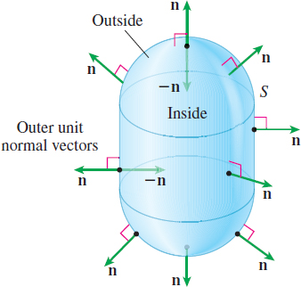
For a closed surface S, that is, a surface that forms the boundary of a closed, bounded solid E in space, such as a sphere, we agree that the positive orientation of S has the unit normal vectors \mathbf{n} to S pointing away from E and that the negative orientation of S has the unit normal vectors -\mathbf{n} to S pointing inward. For closed surfaces S with a positive orientation, the unit normal vectors are called outer unit normal vectors; for closed surfaces S with a negative orientation, the unit normal vectors are called inner unit normal vectors.* See Figure 59.
* Although at first these definitions seem easy, they contain some hidden difficulties. The discussion here and in the next section is limited to simple types of oriented solids E. A discussion of more general solids is found in metric topology.
1032
All curves are orientable, but not all surfaces are orientable. A famous example of a surface that is not orientable is a Möbius strip. See Figure 60. Although it is not immediately apparent, a Möbius strip has only one side and one boundary component. If you were to begin tracing a line on one side of a Möbius strip and continue to follow it once around, you would end on the other side of the strip, that is, the unit normal vector \mathbf{n} now points in the opposite direction.


NOTE
A Möbius strip is formed by taking a long rectangular strip of paper, giving one end a half-twist, and attaching the two ends. The Möbius strip is named after the German mathematician August Möbius (1790–1868).
EXAMPLE 5Finding the \mathbf{k} Component of the Outer Unit Normal Vectors of an xy\,-Simple Surface
Consider the surface S with positive orientation that forms the boundary of the closed, bounded solid E shown in Figure 61. Notice that the surface S can be decomposed into three surfaces, S_{1}, S_{2}, and S_{3}, and that each of the outer unit normal vectors \mathbf{n}_{1}, \mathbf{n}_{2}, and \mathbf{n}_{3} of the three surfaces points away from the solid E enclosed by S.
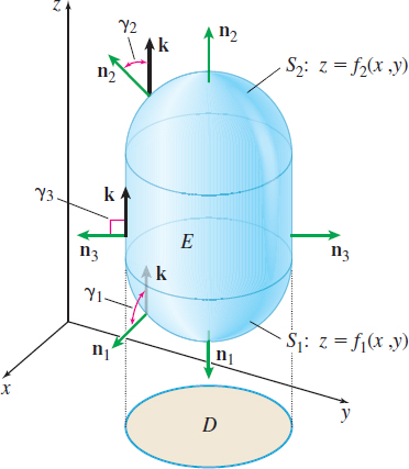
Assume the surfaces S_{1} and S_{2} are defined by the equations \begin{equation*} S_{1}{:}\quad z=f_{1}(x,y)\qquad \hbox{and}\qquad S_{2}{:}\quad z=f_{2}(x,y) \end{equation*}
where f_{1}(x,y)<f_{2}(x,y) on D, the functions f_{1} and f_{2} are continuous on D, and both f_{1} and \ f_{2} have continuous partial derivatives on D. The surface S_{3} is the portion of a cylindrical surface between S_{1} and S_{2} formed by lines parallel to the z-axis and along the boundary of D. The solid E is enclosed by S_{2} on the top, S_{1} on the bottom, and the lateral surface S_{3} on the sides. A surface S with these properties is called \boldsymbol x\boldsymbol y-simple.
Find the \mathbf{k} component of the outer unit normal vectors of S.
Solution For the top surface S_{2}: z=f_{2}(x,y), the outer unit normal vector \mathbf{n}_{2} is the same as the upward-pointing unit normal vector to S_{2}. \begin{equation*} \mathbf{n}_{2}=\dfrac{-(f_{2})_x(x,y)\mathbf{i}-(f_{2})_ y(x,y)\mathbf{j}+\mathbf{k} }{\sqrt{[(f_{2})_x(x,y)]^{2}+[(f_{2})_y(x,y)]^{2}+1}} \end{equation*}
NEED TO REVIEW?
Direction cosines of a vector in space are discussed in Section 10.4, pp. 718-719.
The \mathbf{k} component of \mathbf{n}_{2} is given by the direction cosine \cos \gamma _{2}, where \cos \gamma _{2}=\mathbf{n}_{2}\,{\cdot}\, \mathbf{k}=\dfrac{1}{\sqrt{ [(f_{2})_x(x,y)]^{2}+[(f_{2})_y(x,y)]^{2}+1}}
1033
For the bottom surface S_{1}: z=f_{1}(x,y), the outer unit normal vector \mathbf{n}_{1} equals the downward-pointing unit normal vector -\mathbf{n} to S_{1}. \begin{equation*} \mathbf{n}_{1}=-\mathbf{n}=\dfrac{(f_{1})_{x}(x,y)\mathbf{i}+(f_{1})_y(x,y)\mathbf{j}- \mathbf{k}}{\sqrt{[(f_{1})_x(x,y)]^{2}+[(f_{1})_y(x,y)]^{2}+1}} \end{equation*}
The \mathbf{k} component of \mathbf{n}_{1} is given by the direction cosine \cos \gamma _{1}, where \cos \gamma _{1}=\mathbf{n}_{1}\,{\cdot}\, \mathbf{k}=\dfrac{-1}{\sqrt{[(f_{1})_x(x,y)]^{2}+[(f_{1})_y(x,y)]^{2}+1}}
For the lateral surface S_{3}, the outer unit normal vector \mathbf{n} _{3} is orthogonal to \mathbf{k} at each point on S_{3}. The \mathbf{k } component of \mathbf{n}_{3}, given by the direction cosine, \cos \gamma _{3}, is therefore 0.
EXAMPLE 6Finding the Outer Unit Normal Vectors to a Surface S
Find the outer unit normal vectors to the solid E enclosed by z=f(x,y)=\sqrt{R^{2}-x^{2}-y^{2}}\quad\hbox{and}\quad z=0\qquad 0\leq x^{2}+y^{2}\leq R^{2}
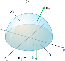
Solution The solid E is the interior of a hemisphere with center at (0,0,0) and radius R as shown in Figure 62. The surface S consists of two surfaces, S_{1} and S_{2}. The bottom surface S_{1} and top surface S_{2} are defined by \begin{equation*} S_{1}{:}\quad z=0 \quad \hbox{and}\quad S_{2}{:}\quad z=f(x,y)=\sqrt{R^{2}-x^{2}-y^{2}}\qquad 0\leq x^{2}+y^{2}\leq R^{2} \end{equation*}
The outer unit normal vector \mathbf{n}_{1} of S_{1} is -\mathbf{k}.
To find the outer unit normal vector \mathbf{n}_{2} of S_{2}, we find f_{x}(x,y) and f_{y}(x,y) . \begin{equation*} f_{x}(x,y)=\dfrac{-x}{\sqrt{R^{2}-x^{2}-y^{2}}}=\dfrac{-x}{z}\qquad \hbox{and} \qquad f_{y}(x,y)=\dfrac{-y}{\sqrt{R^{2}-x^{2}-y^{2}}}=\dfrac{-y}{z} \end{equation*}
Then \begin{eqnarray*} \mathbf{n}_{2}&=&\dfrac{-f_{x}(x,y)\mathbf{i}-f_{y}(x,y)\mathbf{j}+\mathbf{k}}{ \sqrt{[f_{x}(x,y)]^{2}+[f_{y}(x,y)]^{2}+1}}=\dfrac{\dfrac{x}{z}\mathbf{i}+ \dfrac{y}{z}\mathbf{j}+\mathbf{k}}{\sqrt{\dfrac{x^{2}}{z^{2}}+\dfrac{y^{2}}{ z^{2}}+1}}\\ &=&\dfrac{x\mathbf{i}+y\mathbf{j}+z\,\mathbf{k}}{\sqrt{ x^{2}+y^{2}+z^{2}}}=\dfrac{x\mathbf{i}+y\mathbf{i}+z\mathbf{k}}{R} \end{eqnarray*}
NOW WORK
3 Find the Flux of a Vector Field Across a SurfacePrinted Page 1033
An important application of a surface integral measures the rate of flow of a fluid across a surface S, also called the flux across S. Consider solar winds (protons and electrons flowing out of the Sun) as they strike Earth (a spherical surface). The rate of flow of the solar winds across the surface of Earth is an example of flux.
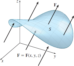
Suppose \mathbf{F}=\mathbf{F}(x,y,z) is a vector field that represents the velocity of a fluid, such as air or water, and suppose \rho =\rho (x,y,z) denotes the variable mass density of the fluid. Then \rho \mathbf{F} equals the rate of flow (mass per unit time) per unit area of the fluid. Let S be an orientable surface immersed in the fluid that does not impede its flow. If \mathbf{n} is a unit normal vector of S, then \rho \mathbf{F}\,{\cdot}\, \mathbf{n} equals the rate of flow of fluid in the direction of \mathbf{n}. See Figure 63.
We seek a formula for the flux across S, that is, the mass of fluid that flows across S in a unit of time.
We begin by partitioning S into n patches S_{i}, i=1,\,2,\,\ldots ,\,n, and concentrate on patch S_{i} whose area is \Delta S_{i}. The mass of fluid per unit time crossing patch S_{i} in the direction of the unit normal \mathbf{n}_{i} is approximately \bbox[5px, border:1px solid black, #F9F7ED]{\bbox[#FAF8ED,5pt]{ \rho \mathbf{F}\,{\cdot}\, \mathbf{n}_{i}\Delta S_{i} } }
1034
where \mathbf{F} is calculated at some point on the patch S_{i}. We define the norm \left\Vert \Delta \right\Vert of the partition to be the largest area \Delta S_{i}. See Figure 64.
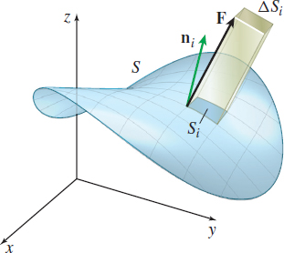
Now we form the sums \sum\limits_{i=1}^{n}\rho \mathbf{F}\,{\cdot}\, \mathbf{n}_{i}\Delta S_{i}
The flux of \mathbf{F} across S, that is, the mass of fluid flowing across the surface S in a unit of time in the direction of \mathbf{n}, is \bbox[5px, border:1px solid black, #F9F7ED]{\bbox[#FAF8ED,5pt]{ \dfrac{\hbox{Mass of fluid}}{\hbox{Unit time}} =\lim\limits_{\Vert \Delta \Vert \rightarrow 0}\sum\limits_{i=1}^{n}\rho \mathbf{F}\,{\cdot}\, \mathbf{n}_{i}\Delta S_{i}=\iint\limits_{\kern-3ptS}\rho \mathbf{F} \,{\cdot}\, \mathbf{n}\,dS }}
provided the limit exists.
EXAMPLE 7Finding the Flux of \mathbf{F} Across a Cylinder
A fluid has a constant mass density \rho . Find the mass of fluid flowing across the cylinder x^{2}+y^{2}=4, where 0\leq z\leq 3, in a unit of time in the direction outward from the z-axis, if the velocity of the fluid at any point on the cylinder is \mathbf{F}=\mathbf{F}(x,y,z)=x\mathbf{i} +y\mathbf{j}+2z\mathbf{k}. That is, find the flux of \mathbf{F} across the cylinder.
Solution In cylindrical coordinates x^{2}+y^{2}=r^{2}=4, or equivalently, r=2, which leads to the parametrization \mathbf{r}\left( \theta ,z\right) =2\cos \theta \,\mathbf{i}+2\sin \theta \,\mathbf{j}+z\,\mathbf{k}, 0\leq \theta \leq 2\pi , 0\leq z\leq 3.
We seek \left\Vert \mathbf{r}_{\theta}\times \mathbf{r}_{z }\right\Vert and dS.
The partial derivatives of \mathbf{r} are \begin{eqnarray*} \mathbf{r}_{\theta }&=&-2\sin \theta \,\mathbf{i}+2\cos \theta \,\mathbf{j}\quad \quad \ \mathbf{r}_{z}=\mathbf{k}\\[4pt] \mathbf{r}_{\theta }\times \mathbf{r}_{z} &=& \left|\begin{array}{c@{\quad}c@{\quad}c} \mathbf{i} & \mathbf{j} & \mathbf{k} \\[3pt] -2\sin \theta & 2\cos \theta & 0 \\[3pt] 0 & 0 & 1 \end{array}\right| =2\cos \theta\, \mathbf{i}+2\sin \theta\, \mathbf{j} \\[4pt] \left\Vert \mathbf{r}_{\theta }\times \mathbf{r}_{z}\right\Vert &=&\sqrt{ 4\cos ^{2}\theta +4\sin ^{2}\theta }=2 \\[4pt] dS &=&\left\Vert \mathbf{r}_{\theta }\times \mathbf{r}_{z}\right\Vert d\theta \,dz=2\,d\theta \,dz \end{eqnarray*}
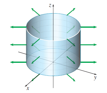
Then the unit normal vector \mathbf{n} is \begin{equation*} \mathbf{n}=\dfrac{\mathbf{r}_{\theta}\times \mathbf{r}_{z}}{\left\Vert \mathbf{r}_{\theta}\times \mathbf{r}_{z}\right\Vert }=\dfrac{2\cos \theta\, \mathbf{i}+2\sin \theta\, \mathbf{j}}{2}=\cos \theta\, \mathbf{i}+\sin \theta\, \mathbf{j} \end{equation*}
These vectors point outward from the surface of the cylinder, so we have the correct orientation. Figure 65 shows the cylinder x^{2}+y^{2}=4, where 0\leq z\leq 3, and the outer unit normal vectors to the cylinder.
We now write \mathbf{F} using the parametrization. \mathbf{F}=\mathbf{F}(x,y,z)=\mathbf{F}(\theta ,z)=2\cos \theta \,\mathbf{i} +2\sin \theta \,\mathbf{j}+2z\,\mathbf{k}
The velocity of the fluid in the direction of \mathbf{n} is \begin{equation*} \mathbf{F\,{\cdot}\, n}=\left( 2\cos \theta \,\mathbf{i}+2\sin \theta \,\mathbf{j} +2z\,\mathbf{k}\right) \,{\cdot}\, \left( \cos \theta\, \mathbf{i}+\sin \theta\, \mathbf{j}\right) =2\cos ^{2}\theta \,+2\sin ^{2}\theta =2 \end{equation*}
The mass of fluid flowing across the cylinder x^{2}+y^{2}=4 in a unit of time in the direction of \mathbf{n} is given by \iint\limits_{\kern-3ptS}\rho \,\mathbf{F}\,{\cdot}\, \mathbf{n}\,dS=\int_{0}^{3} \int_{0}^{2\pi }\left( \rho \,2\right) 2\,d\theta \,dz=4\rho \int_{0}^{3}2\pi \,dz=\left( 8\rho \pi \right) 3=24\rho \pi
The flux of \mathbf{F} across S is 24\rho \pi.
NOW WORK
1035
EXAMPLE 8Finding the Flux of \mathbf{F} Across a Cube
A fluid has constant mass density \rho . Find the mass per unit time of fluid flowing across the cube enclosed by the planes x=0, x=1, y=0, y=1, z=0, and z=1 in the direction of the outer unit normal vectors if the velocity of the fluid at any point on the cube is \mathbf{F}=\mathbf{F} (x,y,z)=4xz\mathbf{i}-y^{2}\mathbf{j}+yz\mathbf{k}. That is, find the flux of \mathbf{F} across the cube.
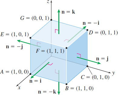
Solution Figure 66 shows the cube and its six faces. The mass per unit time of fluid flowing across the cube in the direction of the outer unit normal vector \mathbf{n} is \iint\limits_{\kern-3ptS}\rho \mathbf{F}\,{\cdot}\, \mathbf{n}\,dS=\rho \iint\limits_{\kern-3ptS} \mathbf{F}\,{\cdot}\, \mathbf{n}\,dS
We decompose S into its six faces and find the surface integral over each one, as shown in Table 1.
| Face | \mathbf{n} | \mathbf{F} | {\bf F} \,{\cdot}\, {\bf n} | \rho \iint\limits_{\kern-3ptS}\mathbf{F}\,{\cdot}\, \mathbf{n}\,dS | |
|---|---|---|---|---|---|
| S_{1}={\it ABCO} | z=0 | -\mathbf{k} | -y^{2}\mathbf{j} | 0 | 0 |
| S_{2}={\it OAEG} | y=0 | -\mathbf{j} | 4xz\mathbf{i} | 0 | 0 |
| S_{3}={\it OCDG} | x=0 | -\mathbf{i} | -y^{2}\mathbf{j}+yz\mathbf{k} | 0 | 0 |
| S_{4}={\it ABFE} | x=1 | \mathbf{i} | 4z\mathbf{i}-y^{2}\mathbf{j}+yz\mathbf{k} | 4z | \rho \int_{0}^{1}\int_{0}^{1}4z\,dy\,dz=2\rho |
| S_{5}={\it BCDF} | y=1 | \mathbf{j} | 4xz\mathbf{i}-\mathbf{j}+z\mathbf{k} | -1 | -\rho \int_{0}^{1}\int_{0}^{1}\,dx\,dz=-\rho |
| S_{6}={\it DFEG} | z=1 | \mathbf{k} | 4x\mathbf{i}-y^{2}\mathbf{j}+y\mathbf{k} | y | \rho\int_{0}^{1}\int_{0}^{1}y\,dx\,dy=\dfrac{1}{2}\rho |
The mass per unit time of fluid flowing across the cube is 0+0+0+2\rho -\rho +\dfrac{1}{2}\rho = \dfrac{3}{2}\rho
NOW WORK
The idea of flux, the rate of flow of a fluid across a surface S, describes many different phenomena. As an example, we consider the flow of electricity across a surface S.
Application: Electric FluxPrinted Page 1035
Suppose \mathbf{E} is an electric field and S is a piecewise-smooth surface with orientation \mathbf{n}. Then the electric flux \Phi _{\mathbf{E}}, the rate at which the electric field passes through S, is given by \begin{equation*} \Phi _{\mathbf{E}}=\iint\limits_{\kern-3ptS}\mathbf{E}\,{\cdot}\, \mathbf{n}\,dS \end{equation*}
Further, suppose we place a point charge of q coulombs (\rm {C}) at the origin. Then the corresponding electric field is \begin{equation*} \mathbf{E}=\left( \dfrac{q}{4\pi \epsilon _{0}}\right) \left( \dfrac{x\mathbf{ i}+y\mathbf{j}+z\mathbf{k}}{(x^{2}+y^{2}+z^{2})^{3/2}}\right) \end{equation*}
The field \mathbf{E} is measured in volts per meter (\rm {V}/\rm {\!m}) and \epsilon _{0}\approx 8.854\times 10^{-12}\rm {C}^{2}/\rm {N}\rm {\!m} ^{2} is the permittivity of free space}.
1036
Now suppose S_{R} is the sphere x^{2}+y^{2}+z^{2}=R^{2}, R>0. If F(x,y,z)=x^{2}+y^{2}+z^{2}, then \mathbf{n}=\dfrac{\nabla \mathbf{F}}{ \left\Vert \nabla \mathbf{F}\right\Vert }=\dfrac{x\mathbf{i}+y\mathbf{j}+z \mathbf{k}}{R} is the outward-pointing unit normal for S_{R}. Then \begin{eqnarray*} \mathbf{E}\,{\cdot}\, \mathbf{n} &=&\left( \dfrac{q}{4\pi \epsilon _{0}}\right) \left( \dfrac{x\mathbf{i}+y\mathbf{j}+z\mathbf{k}}{(x^{2}+y^{2}+z^{2})^{3/2}} \right) \,{\cdot}\, \dfrac{x\mathbf{i}+y\mathbf{j}+z\mathbf{k}}{R} \\[4pt] &=&\left( \dfrac{q}{4\pi \epsilon _{0}}\right) \left( \dfrac{x^{2}+y^{2}+z^{2} }{R^{3}\,{\cdot}\, R}\right) =\dfrac{q}{4\pi \epsilon _{0}}\dfrac{R^{2}}{R^{4}}= \dfrac{q}{4\pi \epsilon _{0}R^{2}} \end{eqnarray*}
Using the fact that the surface area S_{R} of a sphere of radius R is 4\pi R^{2}, we get \begin{equation*} \Phi _{\mathbf{E}}=\iint\limits_{\kern-3ptS_{R}}\mathbf{E}\,{\cdot}\, \mathbf{n} \,dS=\iint\limits_{\kern-3ptS_{R}}\dfrac{q}{4\pi \epsilon _{0}R^{2}}\,dS=\dfrac{q}{ 4\pi \epsilon _{0}R^{2}}\iint\limits_{\kern-3ptS_{R}}1\,dS=\dfrac{q}{4\pi \epsilon _{0}R^{2}}\,{\cdot}\, 4\pi R^{2}=\dfrac{q}{\epsilon _{0}} \end{equation*}
This means that the electric flux of a point charge q originating at the center of a sphere is independent of the size of the sphere.