10.4 The Dot ProductPrinted Page 715
OBJECTIVES
When you finish this section, you should be able to:
When working with vectors there are three types of multiplication. In Sections 10.1 and 10.2, we defined the scalar multiple of a vector v as the product of a scalar and a vector. The resulting product is a vector. Now we discuss the second of the three types of multiplication, the dot product. The dot product is the product of two vectors, but the result is a scalar. In Section 10.5, we investigate the third type of multiplication, called the cross product. One important use of the dot product is to find the angle between two vectors.
DEFINITION Dot Product
If v=v1i+v2j and w=w1i+w2j are two vectors in the plane, the dot product v⋅w is defined as v⋅w=v1w1+v2w2
Similarly, if v=v1i+v2j+v3k and w=w1i+w2j+w3k are two vectors in space, the dot product v⋅w is defined as v⋅w=v1w1+v2w2+v3w3
NOTE
The dot product of two vectors is not a vector. It is a scalar. The dot product is sometimes called the scalar product.
1 Find the Dot Product of Two VectorsPrinted Page 715
EXAMPLE 1Finding the Dot Product of Two Vectors
(a) If v=2i−3j and w=i+j, then v⋅w=(2)(1)+(−3)(1)=2−3=−1w⋅v=(1)(2)+(1)(−3)=2−3=−1v⋅v=22+(−3)2=4+9=13w⋅w=12+12=2
(b) If v=2i−j+k and w=4i+2j−k, then v⋅w=(2)(4)+(−1)(2)+(1)(−1)w⋅v=(4)(2)+(2)(−1)+(−1)(1)=8−2−1=5=8−2−1=5v⋅v=4+1+1=6w⋅w=16+4+1=21
NOW WORK
716
The results from Example 1 suggest some of the properties of the dot product.
THEOREM Properties of the Dot Product
If u, v, and w are vectors and a is any scalar, then:
- Magnitude property: v⋅v=‖
- Commutative property: \bbox[5px, border:1px solid black, #F9F7ED]{ \mathbf{u\,{\cdot}\, v=v\,{\cdot}\, u} }
- Distributive property: \bbox[5px, border:1px solid black, #F9F7ED]{ \mathbf{u}\,{\cdot}\, (\mathbf{v}+\mathbf{w})=\mathbf{u}\,{\cdot}\, \mathbf{v}+\mathbf{u}\,{\cdot}\, \mathbf{w} }
- Linearity property: \bbox[5px, border:1px solid black, #F9F7ED]{ a ( \mathbf{u\,{\cdot}\, v}) =( a\mathbf{u}) \,{\cdot}\, \mathbf{v} }
- Zero-vector property: \bbox[5px, border:1px solid black, #F9F7ED]{ \mathbf{0}\,{\cdot}\, \mathbf{v}=0 }
We prove the magnitude property \mathbf{v}\,{\cdot}\, \mathbf{v}=\left\Vert \mathbf{v} \right\Vert ^{2} and the commutative property for vectors in space. The remaining proofs are left as exercises (see Problems 78-82).
Proof
To show \mathbf{v}\,{\cdot}\, \mathbf{v}=\left\Vert \mathbf{v} \right\Vert ^{2}, we let \mathbf{v}=v_{1}\mathbf{i}+v_{2}\mathbf{j}+v_{3} \mathbf{k}. Then \begin{equation*} \mathbf{v}\,{\cdot}\, \mathbf{v} =v_{1}v_{1}+v_{2}v_{2}+v_{3}v_{3}=v_{1}^{2}+v_{2}^{2}+v_{3}^{2}=\left\Vert \mathbf{v}\right\Vert ^{2} \end{equation*}
Commutative Property: Let \mathbf{u}=u_{1}\mathbf{i}+u_{2}\mathbf{j} +u_{3}\mathbf{k} and \mathbf{v}=v_{1}\mathbf{i}+v_{2}\mathbf{j} +v_{3}\mathbf{k}. Then \mathbf{u}\,{\cdot}\, \mathbf{v} =u_{1}v_{1}+u_{2}v_{2}+u_{3}v_{3}=v_{1}u_{1}+v_{2}u_{2}+v_{3}u_{3}=\mathbf{v} \,{\cdot}\, \mathbf{u}
A consequence of the property \mathbf{v}\,{\cdot}\, \mathbf{v}=\left\Vert \mathbf{ v}\right\Vert ^{2} is that for any vector \mathbf{v}, \bbox[5px, border:1px solid black, #F9F7ED]{ \mathbf{v}\,{\cdot}\, \mathbf{v}\geq 0\quad\hbox{and}\ \quad \mathbf{v }\,{\cdot}\, \mathbf{v}=0\quad\hbox{if and only if}\quad \mathbf{v}=\mathbf{0} }
2 Find the Angle Between Two VectorsPrinted Page 716
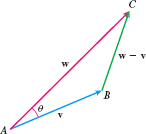
If \mathbf{v} and \mathbf{w} are two nonzero vectors, we can position \mathbf{v} and \mathbf{w} so they have the same initial point. Then the vectors \mathbf{v}, \mathbf{w}, and \mathbf{w-v} form a triangle, as shown in Figure 35. We want to find an expression for the angle \theta between the vectors \mathbf{v} and \mathbf{ w}.
Since the sides of the triangle have lengths \Vert \mathbf{v}\Vert ,\Vert \mathbf{w}\Vert , and \Vert \mathbf{w}-\mathbf{v}\Vert , we can use the Law of Cosines to find the cosine of angle \theta . \begin{equation*} \Vert \mathbf{w}-\mathbf{v}\Vert ^{2}=\Vert \mathbf{v}\Vert ^{2}+\Vert \mathbf{w}\Vert ^{2}-2\Vert \mathbf{v}\Vert \Vert \mathbf{w}\Vert \cos \theta\tag{1} \end{equation*}
Now we use properties of the dot product to write this equation in terms of dot products. Since \mathbf{v}\,{\cdot}\, \mathbf{v}=\Vert \mathbf{v}\Vert ^{2}, we can write (1) in the form \begin{equation*} (\mathbf{w}-\mathbf{v})\,{\cdot}\, (\mathbf{w}-\mathbf{v})=\mathbf{v}\,{\cdot}\, \mathbf{ v}+\mathbf{w}\,{\cdot}\, \mathbf{w}-2\Vert \mathbf{v}\Vert \Vert \mathbf{w}\Vert \cos \theta\tag{2} \end{equation*}
NEED TO REVIEW?
The Law of Cosines states that c^{2}=a^{2}+b^{2}-2ab \cos \theta, where a,b, and c , are the lengths of the sides of a triangle and \theta is the angle opposite the side of length c. The Law of the Cosines is discussed in Appendix A.4, p. A-37.
Now we use the distributive property twice on the term (\mathbf{w}-\mathbf{v })\,{\cdot}\, (\mathbf{w}-\mathbf{v}). \begin{eqnarray*} (\mathbf{w}-\mathbf{v})\,{\cdot}\, (\mathbf{w}-\mathbf{v}) &=&\mathbf{w}\,{\cdot}\, \left( \mathbf{w-v}\right) -\mathbf{v}\,{\cdot}\, ( \mathbf{w-v}) \\[3pt] &=&\mathbf{w\,{\cdot}\, w-w\,{\cdot}\, v-v\,{\cdot}\, w+v\,{\cdot}\, v} \\[3pt] &=&\mathbf{w\,{\cdot}\, w+v\,{\cdot}\, v-2}( \mathbf{v\,{\cdot}\, w}) \end{eqnarray*}
717
We substitute this result back into equation (2) and simplify. This yields \begin{eqnarray*} \mathbf{w\,{\cdot}\, w+v\,{\cdot}\, v} -2 ( \mathbf{v\,{\cdot}\, w}) & =&\mathbf{v} \,{\cdot}\, \mathbf{v}+\mathbf{w}\,{\cdot}\, \mathbf{w}-2\Vert \mathbf{v}\Vert \Vert \mathbf{w}\Vert \cos \theta \\ \mathbf{v}\,{\cdot}\, \mathbf{w}&=& \Vert \mathbf{v}\Vert \Vert \mathbf{w}\Vert \cos \theta \end{eqnarray*}
We have proved the following result.
NOTE
If \mathbf{v}\,{\cdot}\, \mathbf{w} >0, the angle between \mathbf{v} and \mathbf{w} is acute. If \mathbf{v}\,{\cdot}\, \mathbf{w} \lt 0, the angle between \mathbf{v} and \mathbf{w} is obtuse.
THEOREM Angle Between Vectors
The angle \theta , where 0\leq \theta \leq \pi, between two nonzero vectors \mathbf{v} and \mathbf{w} is given by the formula \bbox[5px, border:1px solid black, #F9F7ED]{ \cos \theta =\dfrac{\mathbf{v }\,{\cdot}\, \mathbf{w}}{\Vert \mathbf{v}\Vert \Vert \mathbf{w}\Vert } }
EXAMPLE 2Finding the Dot Product of Two Vectors
Find the angle between the vectors \mathbf{v}=2\mathbf{i}-\mathbf{j}+ \mathbf{k} and \mathbf{w}=- \mathbf{i}+\mathbf{j}.
Solution We find \mathbf{v}\,{\cdot}\, \mathbf{w}, \Vert \mathbf{v} \Vert , and \Vert \mathbf{w}\Vert. \begin{eqnarray*} \mathbf{v}\,{\cdot}\, \mathbf{w} &=&(2) (-1) +(-1) (1) +(1) (0) =-2-1+0=-3 \\[4pt] \Vert \mathbf{v}\Vert &=&\sqrt{2^{2}+(-1) ^{2}+1^{2}}=\sqrt{6} \\[4pt] \Vert \mathbf{w}\Vert &=&\sqrt{(-1) ^{2}+1^{2}}=\sqrt{2} \end{eqnarray*}
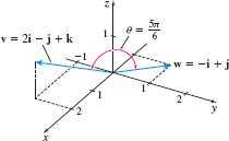
Then if \theta is the angle between \mathbf{v} and \mathbf{w}, \begin{equation*} \cos \theta =\dfrac{\mathbf{v}\,{\cdot}\, \mathbf{w}}{\Vert \mathbf{v}\Vert \Vert \mathbf{w}\Vert }=\dfrac{-3}{( \sqrt{6}) (\sqrt{2}) }= \dfrac{-3}{\sqrt{12}}=-\dfrac{\sqrt{3}}{2} \end{equation*}
Since 0\leq \theta \leq \pi, the angle \theta between \mathbf{v} and \mathbf{w} is \dfrac{5\pi}{6} radians. See Figure 36.
NOW WORK
EXAMPLE 3Finding the True Direction of an Airplane
An airplane has an air speed of 400 km/h and is headed east. Find the true direction of the airplane relative to the ground if there is a northwesterly wind of 80~\text{km}/~\text{h}.
Solution This is the same situation from Example 8 of Section 10.3. There, we found the velocity of the airplane relative to the ground is \mathbf{v}_{\mathrm{g}}=( 400+40\sqrt{2}) \mathbf{i}-40\sqrt{2 }\mathbf{j}.
The angle \theta between \mathbf{v}_{\mathrm{g}} and the vector \mathbf{i} (the positive x-axis) is given by \begin{eqnarray*} \cos \theta &=&\dfrac{\mathbf{v}_{\mathrm{g}}\,{\cdot}\, \mathbf{i}}{\Vert \mathbf{v}_{\mathrm{g}}\Vert \Vert \mathbf{i}\Vert }&=&\dfrac{ 400+40\sqrt{2}}{460.06}\approx 0.9924 \\[5pt] \theta &\approx &\cos ^{-1}(0.9924) \approx 7.07^\circ \end{eqnarray*}
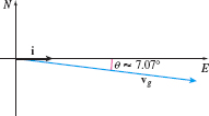
The true direction of the plane is approximately 7.07^\circ south of east. See Figure 37.
NOW WORK
Two nonzero vectors are orthogonal if the angle between them is a right angle (90^\circ). Whether two nonzero vectors are parallel or orthogonal is determined by the angle \theta between the two vectors. \bbox[5px, border:1px solid black, #F9F7ED]{ \begin{array} \hbox~\text{If the angle \(\theta\) between two nonzero vectors \(\mathbf{v}\) and \(\mathbf{ w}\) is \(0\) or \(\pi\), the vectors \(\mathbf{v}\) and \(\mathbf{w}\) are parallel.} \\ \hbox{If the angle \(\theta\) between two nonzero vectors \(\mathbf{v}\) and \(\mathbf{ w}\) is \(\dfrac{\pi }{2}\), the vectors \(\mathbf{v}\) and \(\mathbf{w}\) are orthogonal.} \end{array} }
718
THEOREM Orthogonal Vectors
Two nonzero vectors \mathbf{v} and \mathbf{w} are orthogonal if and only if \bbox[5px, border:1px solid black, #F9F7ED]{ \mathbf{v}\,{\cdot}\, \mathbf{w}=0 }
NOTE
Orthogonal, perpendicular, and normal are all terms that mean “meet at a right angle.” It is customary to refer to two vectors as orthogonal, two lines as perpendicular, and a line and a plane or a vector and a plane as normal.
Proof
We use the formula for the angle between two nonzero vectors, namely \cos \theta =\dfrac{\mathbf{v}\,{\cdot}\, \mathbf{w}}{\left\Vert \mathbf{v}\right\Vert \left\Vert \mathbf{w}\right\Vert }.
If the vectors \mathbf{v} and \mathbf{w} are orthogonal, then the angle \theta between \mathbf{v} and \mathbf{w} is \dfrac{\pi}{2}. Since \cos\dfrac{\pi}{2}=0, it follows that \mathbf{v}\,{\cdot}\, \mathbf{w}=0.
Conversely, if \mathbf{v}\,{\cdot}\, \mathbf{w}=0, then \mathbf{v}=\mathbf{0} or \mathbf{w}=\mathbf{0}, or \cos \theta =0. Since \mathbf{v} and \mathbf{w} are nonzero vectors, \cos \theta =0, so \theta =\dfrac{\pi }{2 } and \mathbf{v} and \mathbf{w} are orthogonal.
3 Determine Whether Two Vectors Are OrthogonalPrinted Page 718
EXAMPLE 4Showing that Two Vectors Are Orthogonal
The vectors \mathbf{v}=2\mathbf{i}-\mathbf{j}+5\mathbf{k} and \ \mathbf{w}=3\mathbf{i}+\mathbf{j}-\mathbf{k} are orthogonal, since \mathbf{v}\,{\cdot}\, \mathbf{w}=6-1-5=0
Since \mathbf{i}\,{\cdot}\, \mathbf{j}=1\,{\cdot}\, 0+ 0\,{\cdot}\, 1=0, the standard basis vectors \mathbf{i} and \mathbf{j} in the plane are orthogonal. The standard basis vectors \mathbf{i}, \mathbf{j}, and \mathbf{k} in space are mutually orthogonal, since \mathbf{i}\,{\cdot}\, \mathbf{j}=0, \mathbf{j}\,{\cdot}\, \mathbf{k}=0, and \mathbf{k}\,{\cdot}\, \mathbf{i}=0.
EXAMPLE 5Making Two Vectors Orthogonal
Find a scalar a so that the vectors \mathbf{v}=2a\mathbf{i}+\mathbf{j}- \mathbf{k} and \mathbf{w}=\mathbf{i}-a \mathbf{j}+\mathbf{k} are orthogonal.
Solution The vectors \mathbf{v} and \mathbf{w} are orthogonal if \mathbf{v}\,{\cdot}\, \mathbf{w}=0. So, \begin{eqnarray*} \mathbf{v}\,{\cdot}\, \mathbf{w}=2a-a-1&=& 0 \\[3pt] a&=& 1 \end{eqnarray*}
The vectors \mathbf{v}=2\mathbf{i}+\mathbf{j}-\mathbf{k} and \mathbf{w}= \mathbf{i}-\mathbf{j}+\mathbf{k} are orthogonal.
NOW WORK
4 Find a Vector in Space from Its Magnitude and DirectionPrinted Page 718
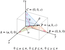
A nonzero vector \mathbf{v} in space can be described by specifying its direction, given by three direction angles \alpha , \beta , \gamma , and its magnitude \left\Vert \mathbf{v}\right\Vert. The direction angles as shown in Figure 38 are defined as \begin{eqnarray*} \alpha & =&\hbox{Angle between }\mathbf{v}\hbox{ and } \mathbf{i}\hbox{, the positive \(x\)-axis}, 0\leq \alpha \leq \pi \\ \beta & =&\hbox{Angle between }\mathbf{v}\hbox{ and } \mathbf{j}\hbox{, the positive \(y\)-axis}, 0\leq \beta \leq \pi \\ \gamma & =&\hbox{Angle between }\mathbf{v}\hbox{ and } \mathbf{k}\hbox{, the positive \(z\)-axis}, 0\leq \gamma \leq \pi \end{eqnarray*}
We seek expressions for \alpha , \beta , and \gamma in terms of the components of a nonzero vector \mathbf{v}. Let \mathbf{v}=v_{1}\mathbf{i} +v_{2}\mathbf{j}+v_{3}\mathbf{k} denote a nonzero vector. The angle \alpha between \mathbf{v} and \mathbf{i}, which lies on the positive x -axis, is given by \begin{equation*} \cos \alpha =\frac{\mathbf{v}\,{\cdot}\, \mathbf{i}}{\Vert \mathbf{v}\Vert \Vert \mathbf{i}\Vert }=\frac{v_{1}}{\Vert \mathbf{v}\Vert } \end{equation*}
Similarly, \begin{equation*} \cos \beta =\dfrac{\mathbf{v\,{\cdot}\, j}}{\left\Vert \mathbf{v}\right\Vert \left\Vert \mathbf{j}\right\Vert }=\frac{v_{2}}{\Vert \mathbf{v}\Vert }\qquad\hbox{and}\qquad \cos \gamma =\dfrac{\mathbf{v\,{\cdot}\, k}}{\left\Vert \mathbf{v}\right\Vert \left\Vert \mathbf{k}\right\Vert }=\frac{v_{3}}{\Vert \mathbf{v}\Vert } \end{equation*}
719
The components of \mathbf{v} are v_{1}=\left\Vert \mathbf{v}\right\Vert \cos \alpha\qquad v_{2}=\left\Vert \mathbf{v}\right\Vert \cos \beta\qquad v_{3}=\left\Vert \mathbf{v}\right\Vert \cos \gamma
THEOREM
If \mathbf{v}=v_{1}\mathbf{i}+v_{2}\mathbf{j}+v_{3}\mathbf{k} is a nonzero vector in space, then \bbox[5px, border:1px solid black, #F9F7ED]{ \begin{array}{l} \cos \alpha =\dfrac{v_{1}}{\sqrt{v_{1}^{2}+v_{2}^{2}+v_{3}^{2}}}=\dfrac{ v_{1}}{\Vert \mathbf{v}\Vert }\qquad \cos \beta =\dfrac{v_{2}}{ \sqrt{v_{1}^{2}+v_{2}^{2}+v_{3}^{2}}}=\dfrac{v_{2}}{\Vert \mathbf{v}\Vert }\\ \cos \gamma =\dfrac{v_{3}}{\sqrt{v_{1}^{2}+v_{2}^{2}+v_{3}^{2} }}=\dfrac{v_{3}}{\Vert \mathbf{v}\Vert } \end{array} } \bbox[5px, border:1px solid black, #F9F7ED]{ \mathbf{v=}\left\Vert \mathbf{v}\right\Vert [ \cos \alpha \mathbf{i} +\cos \beta \mathbf{j}+\cos \gamma \mathbf{k}] }
This result gives the vector \mathbf{v} when its magnitude and direction are known. The numbers \cos \alpha , \cos \beta , and \cos \gamma are called the direction cosines of the vector \mathbf{v}. In Problem 62, you are asked to show that \cos ^{2} \alpha +\cos ^{2}\beta +\cos ^{2}\gamma =1. In other words, the vector \cos \alpha \mathbf{i}+\cos \beta \mathbf{j} +\cos \gamma \mathbf{k} is a unit vector.
EXAMPLE 6Finding the Direction Cosines of a Vector
- (a) Find the magnitude and the direction cosines of \mathbf{v}=-3\mathbf{i }+2\mathbf{j}-6\mathbf{k}.
- (b) Write \mathbf{v} in terms of its magnitude and its direction cosines.
Solution (a) The magnitude of \mathbf{v} is \begin{equation*} \Vert \mathbf{v}\Vert =\sqrt{(-3)^{2}+2^{2}+(-6)^{2}}=\sqrt{49}=7 \end{equation*}
The direction cosines of the vector \mathbf{v} are \cos \alpha =\dfrac{v_{1}}{\left\Vert \mathbf{v}\right\Vert }=\dfrac{-3}{7} \qquad \cos \beta =\dfrac{v_{2}}{\left\Vert \mathbf{v}\right\Vert }= \dfrac{2}{7} \qquad \cos \gamma =\dfrac{v_{3}}{\left\Vert \mathbf{v}\right\Vert }=\dfrac{-6}{7}
(b) Now \mathbf{v=}\left\Vert \mathbf{v}\right\Vert \left[ \cos \alpha {\bf i} + \cos \beta \mathbf{j}+\cos \gamma \mathbf{k}\right] =7\!\left( -\dfrac{3}{7}\mathbf{i}+\dfrac{2}{7}\mathbf{j}-\dfrac{6}{7}\mathbf{k }\right)\! .
NOW WORK
5 Find the Projection of a VectorPrinted Page 719
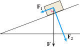
In many applications, it is important to find “how much” of a vector is applied along a given direction. In Figure 39, the force \mathbf{F} due to gravity pulls the block toward the center of Earth. To study the effect of gravity on the block, it is necessary to determine how much of \mathbf{F} is actually pulling the block down the incline (\mathbf{F}_{1}) and how much is pressing the block against the incline (\mathbf{F}_{2}) at a right angle to the incline. Decomposing \mathbf{F} into \mathbf{F}_{1} and \mathbf{F}_{2} allows us to determine when friction is overcome, allowing the block to slide down the incline.
NOTE
The vector \mathbf{v}_{2} orthogonal to \mathbf{w} is sometimes denoted by orth_{\bf w} {\bf v}.
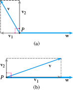
Suppose \mathbf{v} and \mathbf{w} are two nonzero vectors with the same initial point P. We seek to decompose \mathbf{v} into two vectors: \mathbf{v}_{1}, parallel to \mathbf{w}, and \mathbf{v}_{2}, orthogonal to \mathbf{w}. The vector \mathbf{v}_{1} is called the vector projection of \mathbf{v} onto \mathbf{w} and is denoted by proj_{\mathbf{w}}\mathbf{v}. See Figure 40(a) and 40(b) on page 720.
We obtain the vector \mathbf{v}_{1} as follows: We drop a perpendicular from the terminal point of \mathbf{v} to the line containing \mathbf{w}. The vector \mathbf{v}_{1} is the vector from P to the intersection of the line containing \mathbf{w} and the perpendicular. Since \mathbf{v}=\mathbf{v}_{1}+\mathbf{v} _{2}, the dot product \mathbf{v}\,{\cdot}\, \mathbf{w} is \begin{eqnarray*} &&\mathbf{v}\,{\cdot}\, \mathbf{w}\underset{\underset{{\color{#0066A7}{\hbox{\(\mathbf{v=v}_{1}+\mathbf{v}_{2}\)}}}}{\color{#0066A7}{\uparrow}}}{=}(\mathbf{v}_{1}+\mathbf{v}_{2})\,{\cdot}\, \mathbf{w} \underset{\underset{{\color{#0066A7}{\hbox{Distribute}}}}{\color{#0066A7}{\uparrow}}}{=}\mathbf{v}_{1}\,{\cdot}\, \mathbf{w}+\mathbf{v }_{2}\,{\cdot}\, \mathbf{w}\tag{1} \end{eqnarray*}
720
Since \mathbf{v}_{2} is orthogonal to \mathbf{w}, the dot product \mathbf{v}_{2}\,{\cdot}\, \mathbf{w}=0. Since \mathbf{v}_{1} is parallel to \mathbf{w}, there is a scalar a for which \mathbf{v}_{1}=a\mathbf{w}. We make these substitutions in equation (1). \begin{eqnarray*} \mathbf{v}\,{\cdot}\, \mathbf{w} &=&a\,\mathbf{w}\,{\cdot}\, \mathbf{w}+0=a\Vert \mathbf{w}\Vert ^{2} \\[5pt] a &=&\frac{\mathbf{v}\,{\cdot}\, \mathbf{w}}{\Vert \mathbf{w}\Vert ^{2}} \end{eqnarray*}
Then \begin{equation*} \mathbf{v}_{1}=a\mathbf{w}=\frac{\mathbf{v}\,{\cdot}\, \mathbf{w}}{\Vert \mathbf{w} \Vert ^{2}}\,\mathbf{w} \end{equation*}
THEOREM Vector Projection
If \mathbf{v} and \mathbf{w} are two nonzero vectors, the vector projection of \mathbf{v} onto \mathbf{w} is \bbox[5px, border:1px solid black, #F9F7ED]{ \hbox{proj}_{\mathbf{w}}\mathbf{v}=\dfrac{\mathbf{v}\,{\cdot}\, \mathbf{w}}{\Vert \mathbf{w}\Vert ^{2}}\mathbf{w} }
The decomposition of \mathbf{v} into \mathbf{v}_{1} and \mathbf{v}_{2} , where \mathbf{v}_{1} is parallel to \mathbf{w} and \mathbf{v}_{2} is orthogonal to \mathbf{w}, is \bbox[5px, border:1px solid black, #F9F7ED]{ \mathbf{v}_{1}=\dfrac{\mathbf{v}\,{\cdot}\, \mathbf{w}}{\Vert \mathbf{w}\Vert ^{2}}\mathbf{w}\qquad \mathbf{v}_{2}= \mathbf{v-v}_{1} }

EXAMPLE 7Decomposing a Vector into Two Orthogonal Vectors
Find the vector projection of \mathbf{v}=2\mathbf{i}-\mathbf{j}+\mathbf{k} onto \mathbf{w}=\mathbf{i}+\mathbf{j}+\mathbf{k}. Decompose \mathbf{v} into two vectors \mathbf{v}_{1} and \mathbf{v}_{2}, where \mathbf{v} _{1} is parallel to \mathbf{w} and \mathbf{v}_{2} is orthogonal to \mathbf{w}.
Solution We use the formula for the projection of \mathbf{v} onto \mathbf{w}. \begin{eqnarray*} \mathbf{v}_{1}& =&\hbox{proj}_{\mathbf{w}}\mathbf{v}=\frac{\mathbf{v}\,{\cdot}\, \mathbf{w}}{\Vert \mathbf{w}\Vert ^{2}}\mathbf{w} \underset{\underset{\underset{{\color{#0066A7}{\hbox{\(\Vert \mathbf{w}\Vert =\sqrt{1^{2}+1^{2} +1^{2}} =\sqrt{3}\)}}}} {\color{#0066A7}{\hbox{\(\mathbf{v}\,{\cdot}\, \mathbf{w=}2-1+1=2\)}}}} {\color{#0066A7}{\uparrow }}}{=}\frac{2}{(\sqrt{3})^{2}}\mathbf{w}=\frac{2}{3}( \mathbf{i}+\mathbf{j}+\mathbf{k})=\frac{2}{3}\,\mathbf{i}+\frac{2}{3}\, \mathbf{j}+\frac{2}{3}\,\mathbf{k} \\ \mathbf{v}_{2}& =&\mathbf{v}-\mathbf{v}_{1}=(2\mathbf{i}-\mathbf{j}+\mathbf{k} )-\left( \frac{2}{3}\,\mathbf{i}+\frac{2}{3}\,\mathbf{j}+\frac{2}{3}\, \mathbf{k}\right) =\frac{4}{3}\,\mathbf{i}-\frac{5}{3}\,\mathbf{j}+\frac{1}{3 }\,\mathbf{k} \end{eqnarray*}
NOW WORK
6 Compute WorkPrinted Page 720
Work is defined as the energy transferred to or from an object by a force acting on the object.
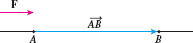
The work W done by a constant force \mathbf{F} in moving an object from A to B along a straight line in the direction of \mathbf{F} is defined to be W=\Vert \mathbf{F}\Vert \Vert \skew5\overrightarrow{\it AB}\Vert \qquad {\color{#0066A7}{\hbox{Work \(=\) force } {\times} \hbox{ distance}}}
In this definition, it is assumed that the constant force \mathbf{F} is applied along the line of motion \skew5\overrightarrow{\it AB}, as shown in Figure 41.
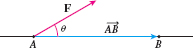
If the constant force \mathbf{F} is not along the line of motion, but instead is at an angle \theta to the direction of motion, as in Figure 42, then the work W done by \mathbf{F} in moving an object from A to B is defined as the dot product. \bbox[5px, border:1px solid black, #F9F7ED]{ W=\mathbf{F}\,{\cdot}\, \skew5\overrightarrow{\it AB} }
721
This definition is compatible with the force times distance definition, since \begin{eqnarray*} W& =&(\hbox{Amount of force in the direction of }\skew5\overrightarrow{\it AB})(\hbox{ distance}) \\[4pt] & =& \Vert \hbox{proj}_{\skew5\overrightarrow{\it AB}} \mathbf{F} \Vert \Vert \skew5\overrightarrow{\it AB} \Vert = \left[ \dfrac{\mathbf{F}\,{\cdot}\, \skew5\overrightarrow{\it AB}}{ \Vert \skew5\overrightarrow{\it AB} \Vert ^{2}} \Vert \skew5\overrightarrow{\it AB} \Vert \right] \Vert \skew5\overrightarrow{\it AB} \Vert =\mathbf{F}\,{\cdot}\, \skew5\overrightarrow{\it AB} \end{eqnarray*}
EXAMPLE 8Computing Work
Find the work done by a force of 2 newtons (N) acting in the direction \mathbf{i}+\mathbf{j}+\mathbf{k} in moving an object 1 m from (0, 0, 0) to (1, 0, 0).
Solution We need to express the force \mathbf{F} in terms of its magnitude and direction. The unit vector \mathbf{u} in the direction \mathbf{v}=\mathbf{i}+\mathbf{j}+\mathbf{k} is \mathbf{u}=\dfrac{\mathbf{v}}{\left\Vert \mathbf{v}\right\Vert }=\dfrac{ \mathbf{i}+\mathbf{j}+\mathbf{k}}{\sqrt{3}}=\dfrac{1}{\sqrt{3}}\mathbf{i}+ \dfrac{1}{\sqrt{3}}\mathbf{j}+\dfrac{1}{\sqrt{3}}\mathbf{k}
Since the force vector \mathbf{F} has magnitude 2, we have \mathbf{F}=2\left( \frac{1}{\sqrt{3}}\mathbf{i}+\dfrac{1}{\sqrt{3}}\mathbf{j} +\dfrac{1}{\sqrt{3}}\mathbf{k}\right) =\dfrac{2}{\sqrt{3}}( \mathbf{i}+ \mathbf{j}+\mathbf{k})
The line of motion of the object from ( 0,0,0) to \left( 1,0,0\right) is \skew5\overrightarrow{\it AB}=\mathbf{i}. The work W is therefore W=\mathbf{F}\,{\cdot}\, \skew5\overrightarrow{\it AB}=\frac{2}{\sqrt{3}}(\mathbf{i}+\mathbf{j }+\mathbf{k})\,{\cdot}\ \mathbf{i}=\frac{2}{\sqrt{3}}\hbox{ joules}
RECALL
1 joule =1 newton\cdotmeter; 1~\text {J} =1~\text {N}\cdot\ \text{m}.
NOW WORK
EXAMPLE 9Computing Work
Figure 43 shows a man pushing on a lawn mower handle with a force of 30 lb. How much work is done in moving the lawn mower a distance of 75 ft if the handle makes an angle of 60^{\circ } with the ground?
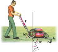
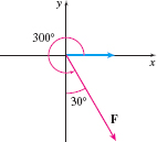
Solution We set up the coordinate system so that the lawn mower is moved from (0,0) to (75,0). Then the motion occurs along \skew5\overrightarrow{\it AB}=75\,\mathbf{i}. The force vector \mathbf{F}, as shown in Figure 44, makes an angle of 300^\circ to the positive x-axis. Since \Vert \mathbf{F} \Vert = 30, \mathbf{F} is given by \begin{equation*} \mathbf{F}=30[ (\cos 300^{\circ })\mathbf{i}+(\sin 300^{\circ })\mathbf{ j}] =30\left[ \dfrac{1}{2}\mathbf{i}-\dfrac{\sqrt{3}}{2}\mathbf{j} \right] =15\mathbf{i}-15\sqrt{3}\mathbf{j} \end{equation*}
Then the work W done is W=\mathbf{F}\,{\cdot}\, \skew5\overrightarrow{\it AB}=(15\mathbf{i}-15\sqrt{3}\mathbf{j} )\,{\cdot}\, 75\mathbf{i}=1125 \hbox{ft-lb}